Beyond Discrete Support in Large-scale Bayesian Deep Learning
Blog post to accompany Radial Bayesian Neural Networks at AI STATS 2020. Sebastian Farquhar, Michael Osborne, Yarin Gal.
Most neural networks learn a single estimate of the best network weights. But, in reality, we are unsure. What we really want is to learn a probability distribution over those weights that reflects our uncertainty, given the data. This is called the posterior probability distribution over the weights of the network. A distribution leaves open the possibility of improving our inference when we get more data through Bayesian updating, e.g. by continual learning. Beyond that, it makes it easy to estimate the uncertainty of our predictions.
Successful methods like Monte Carlo Dropout or Deep Ensembles have already shown how uncertainty quantification can be used for interesting applications. But Bayesian updating is hard for these methods (because they have “discrete support”).
Mean-field variational inference (MFVI) is a practical method that is straightforward to use for Bayesian updating. MFVI is also called Bayes-by-Backprop (BBB) when used with the reparametrisation trick. But if you sit down and try to use it with large models you will find many challenging pitfalls in practice (like unstable optimisation).
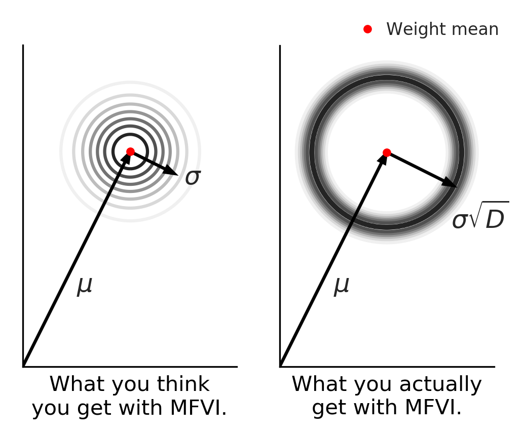
In this post we try to shed light on why MFVI/BBB fails, and in the process introduce Radial Bayesian Neural Networks (BNNs). Radial BNNs give us a simple new view on the mean-field variational inference approximation for neural networks. They work by fixing the weird behaviour of high-dimensional multivariate Gaussians used in MFVI/BBB. Intuitively, we imagine these Gaussians produce a distribution over models that has high density near the mean and falls off away from the mean, like the left-hand side figure above, which shows a 2-D projection of the high-dimensional space. But in fact, the real distribution has most of the density in a “soap-bubble” far from the mean, like the right-hand side. Radial BNN’s recover the distribution that we intuitively imagine when we use a Gaussian.
Despite their simplicity, Radial BNNs work surprisingly well in big models with 15M+ parameters, and solve many of the problems we had before with mean-field. We show that Radial BNNs support both Bayesian updating (continual learning) and uncertainty quantification better than popular alternatives like mean-field variational inference, deep ensembles, or Monte Carlo (MC) dropout.
Read the full paper (arXiv link).
Why be Bayesian about Neural Networks?
(If you’re already sold on Bayesian deep learning and don’t need more convincing, skip to our discussion of what can go wrong with standard mean-field variational inference.)
Uncertainty Quantification
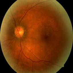
To ground the discussion, let’s think about an example from medical imaging, diabetic retinopathy in particular. One complication of diabetes is retinopathy, damage to the retina which is the leading cause of blindness in working age people. Diagnosis can be made by examining a “fundus” image, a kind of picture of the retina.
A healthy eye might look like this:
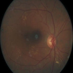
Disease could look a little different, notice the spots on the image which reflect damage:
But sometimes the image just has camera artefacts. For example, on this one spots appear which are just a problem with the camera:
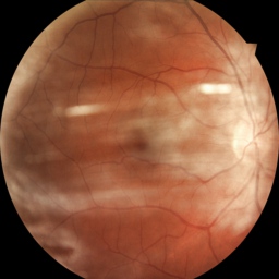
Imagine we’d like to automate this diagnosis. A human optometrist can tell the difference between disease and faulty equipment as second nature. But neural networks are generally not equipped to handle this sort of ‘out-of-distribution’ data. What we’d really like to do is notice the image is bad and take a fresh one. Bayesian neural networks, because they have distributions over the weights, also produce distributions over predictions. This lets us estimate the model’s uncertainty about its prediction and react to it.
Bayesian Updating and Continual Learning
Another nice thing about Bayesian inference is that we can perform “Bayesian updating”. Imagine we’ve already inferred a distribution over weights based on a first dataset using Bayes’ rule. This can be written:
\[p(\theta|\mathcal{D}_1) = \frac{p(\mathcal{D}_1|\theta)p(\theta)}{p(\mathcal{D}_1)}\]where we use the data likelihood, prior, and marginal likelihood of the data to infer the posterior over the weights given our data.
So long as we keep this full distribution (rather than throwing almost all of it away and keeping a point estimate like in ordinary neural networks) we can do another step of inference based on a new dataset. All we have to do is use the posterior that we learned from the first dataset as a prior when learning from the second dataset.
\[p(\theta|\mathcal{D}_1, \mathcal{D_2}) = \frac{p(\mathcal{D}_2|\theta, \mathcal{D}_1)p(\theta|\mathcal{D}_1)}{p(\mathcal{D}_2)}.\] In principle, this is an incredibly powerful tool for learning continuously, rather than retraining from scratch on any problem.
Why care about full-suport methods?
Right now, the tools for Bayesian deep learning are limited. Methods like Monte-Carlo Dropout, Deep Ensembles, SG-MCMC scale pretty well to big models, but unfortunately the output of the learning procedure has what we call “discrete support”. That is, the output assigns exactly zero probability almost everywhere in weight-space. That is implausible a priori, represents extreme over-confidence (no amount of new data can ever update away from exactly zero probability).
For this reason, you can’t use a discrete support method for Bayesian updating! The posterior you get after training on the first dataset, \(p(\theta|\mathcal{D}_1)\) assigns zero probability almost everywhere. So if you try to use it as a prior for further inference, the new posterior distribution has to be zero almost everywhere too, ignoring the new data.
A discrete support method like MC Dropout, SG-MCMC, or Deep Ensembles can't be used as a prior for further inference.
Instead you can use variational inference (VI) with the “mean-field” assumption. People have looked into richer approximate posteriors as well, but these are too expensive at the moment for big models [e.g., 1 2 3]. This method has full support over the whole of weight-space. As a result, it can be used as a prior for futher inference, e.g., in continual learning.
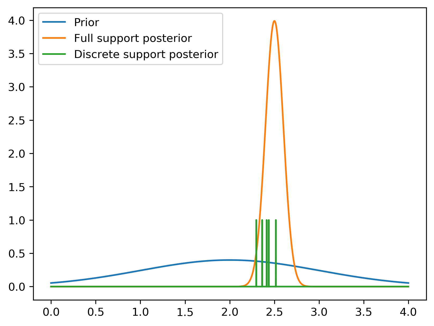
To visualize this, consider the (very simplified) hypothetical posterior inference in the figure above. We start with some broad prior (in blue). After seeing some data, we learn a tighter distribution. In orange is a full support posterior distribution given some hypothetical data. In green, a discrete support posterior distribution. It assigns all its mass at a finite number of points (like if you do MC dropout, Deep Ensembles, or SG-MCMC). This means that if you tried to do further inference, no amount of data could ever inform you about the new posterior probability anywhere except those points.
Unfortunately, MFVI turns out to be quite finicky and dependent on hacks in big models.
Mean-field and Bayes By Backprop Fail in Big BNNs Because of the “Soap Bubble”
Why does mean-field (and Bayes By Backprop) fail with large models?
In few dimensions, Gaussians behave similarly to how you would expect.
In high dimensions, Gaussians do not behave at all how you would expect.
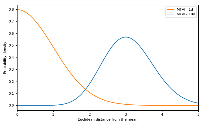
Multivariate Gaussians (and many other distributions) behave unintuitively in high-dimensional spaces. While the Gaussian probability density function becomes small away from the origin, in high dimensional spaces there is much more space (relative to density) as you get further from the origin. This means that for a high-dimensional multivariate Gaussian the probability density along the radius from the origin becomes sharply peaked at a fixed radius from the origin. For relatively small numbers of dimensions, this effect is quite manageable. Here we can see a one-dimensional multivariate Gaussian compared with a 10-dimensional one.
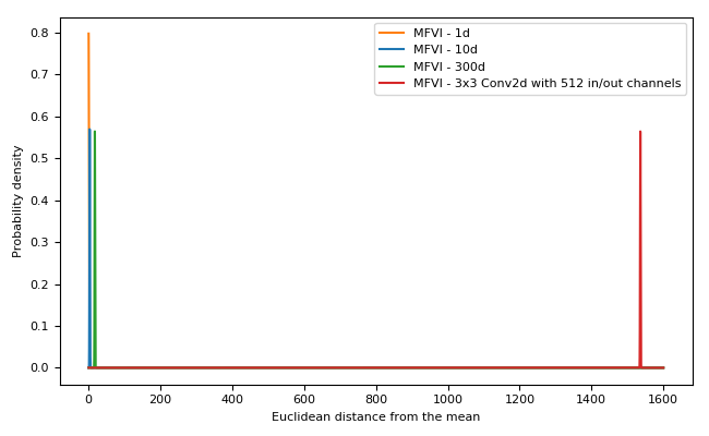
But when we increase the number of dimensions to the point common in neural networks the situtation becomes extreme! For example, consider the graph showing a multivariate Gaussian with the dimensionality of a single 3x3 convolutional layer with 512 input and output channels: in high dimensions the Euclidean distance from the mean of a typical sample is tightly clustered very far from the mean.
The consequence: samples from a high dimensional multivariate Gaussian approximate posterior (the normal Bayes-by-backprop set-up) are clustered in a hyperspherical “soap-bubble” far from the origin.

What you expect is not what you get for multivariate Gaussians. Radial BNNs actually behave how we intuit a Gaussian ought to.
Remember this visualization from before? Mentally, when you picture sampling multivariate noise you might imagine something like the figure on the left in this 2-d projection of the density of samples of your high-dimensional model. Most samples are near the mean and get less likely the further from the model you are. But in fact, the distribution is more like the picture on the right! Almost all samples are compressed in a narrow band far from the mean. Our method can be thought of as giving you back what you intuitively expected your sampling distribution was doing.
In high-dimensional spaces the soap-bubble pathology in ordinary MFVI has the added consequence that almost every sample from the Gaussian is equally far from all the others. What this means is that no sample from your approximate posterior is really representative of your distribution: the result is high variance gradient estimates whenever you train your model away from a tiny initialized variance.
This failure gave rise to a variety of tricks and tweaks to the objective, optimiser, and initialisation. Some change the weight of the KL penalty term for different epochs, while others schedule the learning rate of the optimiser for certain parameters (like posterior variance) so they don’t increase “too much”. People also try to encourage the posterior variance to stay small by initialising it with tiny values, and making sure to stop optimisation before they become too big.
If you don’t do this, you get the bizarre phenomenon for MFVI where training accuracy decreases over time.
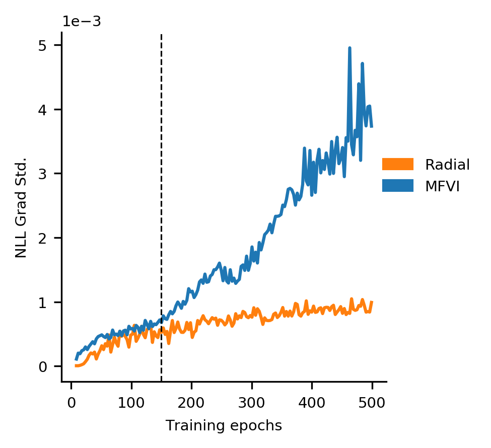
As the sigma parameter grows from its tiny initialization, the gradient variance explodes.
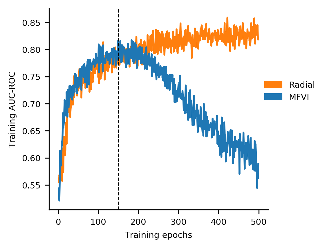
At exactly the same time, the training accuracy starts to fall.
Luckily, we can fix this pathology rather easily. We build on tractable mean-field variational inference, but make a principled adjustment to the approximate posterior distribution. Our approximate posterior adjustment avoids the need for hacky tweaks or endless hyperparameter optimization, and is also tractable in really big networks. At the same time, we keep the full-support probability distributions at the end of training which methods like deep ensembles, MC dropout, or stochastic gradient MCMC throw away. We do this by setting an approximate posterior distribution that has better high-dimensional sampling properties than the typical mean-field multivariate Gaussian.
If you want to skip ahead, you can check out:
- How Radial BNNs use a different approximate posterior to side-step the soap-bubble and keep gradient variance down.
- Experiments showing better accuracy than MC Dropout and Deep Ensembles, better calibration, and how Radial BNNs can be used for continual learning.
- The pros and cons of various approaches to Bayesian Deep Learning.
- How to implement Radial BNNs fast, including a ready-to-use github repo.
Variational Inference that ‘Just Works’ in Big BNNs
Radial BNNs extend on Bayes-by-backprop, a form of Variational Inference (VI).
For VI, we learn an approximate posterior distribution over the weights of the neural network \(q(\mathbf{w})\) and try to minimize the KL-divergence between \(q(\mathbf{w})\) and the true posterior \(p(\mathbf{w}|\mathcal{D})\). Minimizing the KL-divergence can be motivated as a bound on the model evidence or simply by observing that the KL-divergence goes to zero when the approximate posterior and true posterior are identical. (You can read this detailed introduction to variational inference in neural networks for more.)
Bayes-by-backprop (BBB) uses a multivariate Gaussian approximate posterior and makes the extra assumption that each weight distribution is independent of all the others.
\[q(\mathbf{w})_{\text{BBB}} = \prod_i q(w_i)\]where \(w_i \sim \mathcal{N}(\mu_i, \sigma^2_i)\).
BBB distinguishes itself from normal mean-field VI by applying the reparameterization trick using a scaled unit noise random variable and ‘deterministic’ variational parameters:
\[q(\mathbf{w})_{\text{BBB}} = \boldsymbol{\mu} + \boldsymbol{\sigma} \cdot \boldsymbol{\epsilon}_{\text{BBB}}\]where \({\epsilon_{\text{BBB}}}_i \sim \mathcal{N}(0, 1)\).
The change that we make is to replace this approximate posterior distribution with one that is normalized in the following way:
\[\boldsymbol{\epsilon}_{\text{Rad}} = \frac{\boldsymbol{\epsilon}_{\text{BBB}}}{\lVert \boldsymbol{\epsilon}_{\text{BBB}}\rVert} \cdot r\]where \(r \sim \mathcal{N}(0,1)\) (we’ll refer to this as the Radial BNN approximate posterior).
What does this normalization do? The fraction \(\frac{\boldsymbol{\epsilon}_{\text{BBB}}}{\lVert \boldsymbol{\epsilon}_{\text{BBB}}\rVert}\) projects the noise uniformly onto a hypersphere in weight-space while the term \(r\) places a normal distribution over the distance of a sample from the mean.
Radial BNNs Fix Gradient Variance
The Radial BNN approximate posterior does not have the gradient variance problem because we pick a distribution that actually behaves like our intuitive picture of what a multivariate Gaussian should be doing but isn’t.
Remember our noise distribution?
\[\boldsymbol{\epsilon}_{\text{Rad}} = \frac{\boldsymbol{\epsilon}_{\text{BBB}}}{\lVert \boldsymbol{\epsilon}_{\text{BBB}}\rVert} \cdot r\] When we plot the probability density function along the radius, there is no soap bubble no matter how many dimensions we pick. That’s not an accident. Even though it’s easy to write our approximate posterior noise distribution as a normalized multi-variate Gaussian, it is in fact a distribution expressed in hyperspherical coordinates (the N-dimensional generalization of polar coordinates).
In three dimensions that coordinate system looks like this:
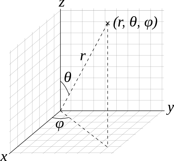
Visualization of spherical coordinates from Wikipedia produced by Dmcq.
Where the radius (r) is the Euclidean distance from the origin, and then two angles specify the direction to travel from the origin to get to the point.
And in the N-dimensional version of this coordinate system, our new noise distribution is:
- Unit Gaussian distribution over the radius.
- Uniform distribution over the surface of the hypersphere in N-space.
As a result, typical samples from the distribution can always be relatively close to the mean in Euclidean space no matter how high-dimensional the model.
In practice, we can show that this leads to lower gradient variance, even for very large models.
Experiments: Radial BNNs Don’t Fail in Big Models (And Outperform SOTA)
Because Radial BNNs fix the variance problems caused by the soap-bubble, they outperform Bayes-by-backprop (even if BBB uses the standard tricks), and even MC Dropout. They even outperform Deep Ensembles, generally regarded as state-of-the-art for many practical uncertainty quantification tasks.
Accuracy
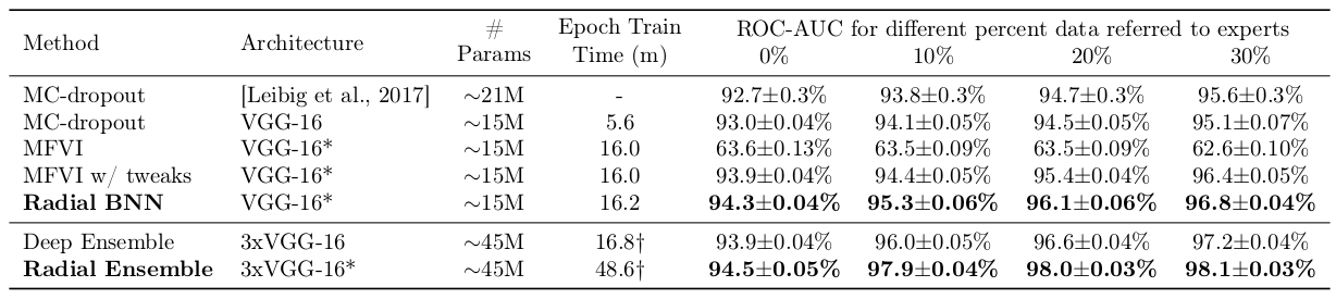
We tested Radial BNNs on the Diabetic Retinopathy task for Bayesian deep learning: a medical imaging task for 512x512 images using a VGG-like architecture. In all cases we use a shrunk version of the model for Radial BNNs and BBB to account for the fact that they need twice as many parameters per weight (both mean and variance).
We test the model’s area under the receiver-operating characteristic curve (AUC-ROC) which is a measure of accuracy which is better suited to unbalanced datasets like the Diabetic Retinopathy dataset.
We also test the uncertainty quantification by not classifying the most uncertain points. If the model is right about where it is most uncertain, the accuracy should go up when they are not evaluated.
When all the data are evaluated, Radial BNNs are better than any of the baselines.
Deep Ensembles have slightly better uncertainty quantification than a single Radial BNN model, but when we consider an ensemble of Radial BNNs with the same number of parameters, they beat Deep Ensembles again.
Calibration
We can also look at the calibration of the models. If a model is well-calibrated, it is right about 50% of the time it classifies something with 50% confidence. Radial BNNs are better calibrated than any of the baselines.
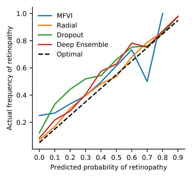
Radial BNNs are more calibrated than other deep methods.
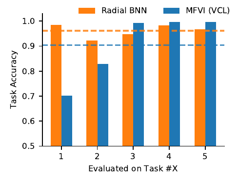
Radial BNNs make continual learning more possible than MFVI networks.
Continual Learning
And because Radial BNNs give you a fully supported approximate posterior (unlike MC Dropout, Deep Ensembles, or SG-MCMC, say) they can be used to do Bayesian updating. We find that a Radial BNN version of the Variational Continual Learning algorithm preserves task accuracy in a sequential continual learning experiment much better than the default version that uses mean-field VI (MFVI). You can see the paper for more experiments and details. Note though, that even with our improvement, the continual learning problem is very difficult, and is still not solved.
Pros and Cons of BNN Approaches
Different approaches to Bayesian deep learning have a variety of advantages, independently of their accuracy and uncertainty quantification. Although we think that Radial BNNs are often the right choice, or at least worth trying, there are definitely settings where you may be best served by a different method.
| Architecture | Model size | Epoch training time | Cost per test example | Full- or discrete-support |
|---|---|---|---|---|
| Radial BNNs | 2 params per weight | ~ | \(K\) forward passes | full |
| Mean-field VI (BBB) | 2 params per weight | ~Radial BNN | \(K\) forward passes | full |
| MC Dropout | 1 param per weight (+ dropout probabilities) | ~\(\frac{\text{Radial BNN}}{3}\) | \(K\) forward passes | discrete |
| Deep Ensemble of \(K\) models | \(K\) params per weight | ~\(\frac{K \cdot \text{Radial BNN}}{3}\) | \(K\) forward passes | discrete |
| SG-MCMC with \(K\) samples | \(K\) params per weight (MCMC samples) | run till you mix | \(K\) forward passes | discrete |
Model size
Radial BNNs and BBB both roughly double the model size for the same architecture because we need to store both mean and variance parameters. For this reason all our mean-field experiments use smaller BNN models when comparing to MC Dropout so that the total number of parameters is held constant. MC Dropout needs to optimize the dropout probabilities and requires a small number of extra parameters for these. Deep Ensembles need to train and store multiple models, which increases the effective model size by \(K\) (often 3-5). SG-MCMC methods also produce multiple samples from the posterior and then need to store them all, increasing the effective model size for inference.
Epoch training time
The various methods converge at different speeds, but the epoch training time for Radial BNNs and BBB are similar and about 3x longer than e.g. Dropout (most of the extra time is spent sampling from multivariate Gaussians, which is not well-optimized on modern GPUs but is an active area for research). Balancing this is the fact that Deep Ensembles must train K models, and therefore execute K times more epochs than Dropout. To a somewhat lesser degree, obtaining samples using SG-MCMC requires some noise generation and also longer training than normal to generate uncorrelated samples from the posterior. However, we have not done a timed comparison to any specific implementation.
Cost per test example and per posterior sample
All methods require a fixed test-time cost of \(K\) forward passes per test example. However, there is an important distinction between Radial BNNs, BBB, and MC Dropout on the one hand and Deep Ensembles and SG-MCMC on the other. The former group explicitly represent a distribution and can generate new samples from that distribution very cheaply. To get more samples from the latter group, we’d need access to the original data to optimize new models with respect to that data. This makes it considerably harder to adaptively use more samples from the posterior to improve accuracy at inference time.
Full or discrete-support
Radial BNNs and mean-field VI have the significant advantage of using a probability distribution which fully covers the weight space. The approximate posteriors that you get from the other approaches are either discrete because of the Bernoulli distribution (MC Dropout) or because the approximate posterior for inference uses an empirical distribution over finitely many point samples (SG-MCMC or Deep Ensembles). A full-support distribution lets you use the approximate posterior from one dataset as a prior for future inference: it enables Bayesian updating. For certain applications, like continual learning, that could be essential.
Putting Radial BNNs in Your Code
Radial BNNs (github repo) are extremely easy to work into whatever code you are already using to perform variational inference.
Sampling from the posterior is a small change. Instead of drawing one sample from your noise distribution:
def bbb_posterior_sample(size):
    return torch.randn(size)
you can instead run:
def radial_posterior_sample(size):
    bbb_epsilon = torch.randn(size)
    radial_distance = torch.randn((1))
    return bbb_epsilon / torch.norm(bbb_epsilon, p=2) * radial_distance
We find that this increases the training time for an epoch by ~1% relative to BBB, but because Radial BNNs are much less sensitive to hyperparameters you can pick a good training setup much faster overall.
In our github repo, we have a fuller version of the code with:
- Batching over both training data and samples from the posterior;
- Pytorch
Moduleobjects that can be called just like vanilla pytorch Layers (Linear, Conv2D, MaxPool2D, GlobalMaxPool2D, and GlobalMeanPool2D); - Automatically computing the correct variational inference loss for the new posterior;
- Modular training script with pre-configured models (toy MLP, VGG-16);
- Ready-to-go config files for MNIST, FashionMNIST, Diabetic Retinopathy;
- Runs vanilla BBB with a single argument switch so it is easy for you to compare to a baseline.
Using the repo, you can quickly implement a pytorch model exactly like you would normally. For example, here is how you would implement an MLP.
class Radial_MNIST_MLP(Module):

    def __init__(self, args):
        super(Radial_MNIST_MLP, self).__init__()

        self.first_layer = Radial_Linear(784, 200, *args)
        self.hidden_layer = Radial_Linear(200, 200, *args)
        self.last_layer = Radial_Linear(200, 10, *args)

    def forward(self, x):
        # Input has shape [examples, samples, height, width]
        x = x.view(x.size()[0], x.size()[1], -1)
        x = F.relu(self.first_layer(x))
        x = F.relu(self.hidden_layer(x))
        x = F.log_softmax(self.last_layer(x), dim=-1)
        return x
where the args could be, for example,
initial_rho = -4  # This is a reasonable value, but not very sensitive.
initial_mu_std = "he"  # Kaiming He init.
variational_distribution = "radial"  # You can use 'gaussian' for normal MFVI.
prior = {
    "name": "gaussian_prior",
    "sigma": 1.0,
    "mu": 0,
}  # Just a unit Gaussian prior.
And then you just run a fairly standard training loop
train_loader = MNISTDataLoader("data", stage="training")
model = Radial_MNIST_MLP()

# We need to set a couple extra values to make sure that the ELBO is calculated right.
loss = Elbo(binary=False, regression=False)
loss.set_model(model, batch_size)
loss.set_num_batches(len(train_loader))

optimizer = torch.optim.Adam(model.parameters())
device = "cuda"
variational_samples = 8  # Sets number of samples from model to use per forward pass

model = model.to(device)
for epoch in range(10):
    for batch_idx, (data, target) in enumerate(train_loader):
        data, target = data.to(device), target.to(device)

        # We tile the data to efficiently parallize forward passes through multiple
        # samples from the variational posterior
        data = data.expand((-1, variational_samples, -1, -1))

        optimizer.zero_grad()
        output = model(data)  # Output has shape [examples, samples, classes]
        nll_loss, kl_term = loss.compute_loss(output, target)
        batch_loss = nll_loss + kl_term
        batch_loss.backward()
        optimizer.step()