Is Mean-field Good Enough for Variational Inference in Bayesian Neural Networks?

Sebastian Farquhar, Lewis Smith, Yarin Gal, 29 Nov 2020

Tl,dr; The bigger your model, the easier it is to be approximately Bayesian.

Blog post accompanying Liberty or Depth: Deep Bayesian Neural Nets Do Not Need Complex Weight Posterior Approximations by Sebastian Farquhar, Lewis Smith, and Yarin Gal at OATML Oxford.

When we do variational inference in Bayesian Neural Networks, we try to learn an approximate distribution over the weights of the neural network that is as close as possible to the true posterior distribution implied by Bayes’ rule and our data. In order to make this tractable, we often like to make the “mean-field” assumption. That is, we assume that each weight in the neural network is independent of all the others. For the commonly used Gaussian approximate posterior, this means that the covariance matrix for the weights is diagonal.

We almost have to do this for big neural networks. The time complexity under this mean-field assumption is linear in the number of parameters — \(\mathcal{O}(n)\) — but modelling the interactions between the weight distributions can be much more expensive. Using a Gaussian with full covariance matrix has a time complexity \(\mathcal{O}(n^6)\) in the number of parameters! (Inverting a full covariance matrix is much more expensive than inverting just the diagonal.)

The trouble is, we’ve generally assumed that the mean-field assumption is lousy. We don’t know a lot about the true posterior distribution over the weights of our model — what we would get if we could properly update our weight distribution with Bayes’ rule — but it seems plausible the weights would have correlations between each other.

In a seminal paper, David MacKay wrote about how bad the mean-field assumption was in Bayesian neural networks:

The diagonal approximation is no good because of the strong posterior correlations in the parameters.

A lot of other researchers since then have taken this for granted, and have put a lot of work into structured covariance approximations which are able to model some of the correlations between the parameters fairly cheaply. But these are all still more expensive than mean-field. Most of the experiments that show them beating mean-field are in smaller models, partly because they are expensive. What if we make the network bigger?

Read the full paper.

Why we should care: Bayes at scale

This is more than just idle curiosity. Bayesian methods offer a lot: more robust prediction, better generalization, reasonable uncertainty. But they are perceived as being too expensive to run, or hard to implement. This stops people from deploying them at scale.

But the key takeaway from this paper should be: the bigger your model, the easier it becomes to be approximately Bayesian.

So as researchers, we’re doing all this work to get better Bayesian approximations, but if we just used simple approximations in big models the problem solves itself. (And gets replaced by other problems: scaling this stuff to huge models comes with its own difficulties, e.g., gradient variance.)

Some empirical observations

We’re going to start with some experiments, which motivate the idea that mean-field variational inference works surprisingly well in big models, especially deeper ones. Later, we’ll think about possible reasons why. There, we also introduce some new analytical tools for exploring piecewise-linear neural networks extending recent work by Adi Shamir, and bridging results from linear models onto non-linear neural networks.

Investigating the true posterior

Above, MacKay (and the others since) began with an assumption: that there are “strong posterior correlations in the parameters”. Is that true?

It is hard to know, especially in large models. But we can get some insight with Hamiltonian Monte Carlo, a relatively expensive tool for getting high quality samples from the true posterior distribution (details in the paper).

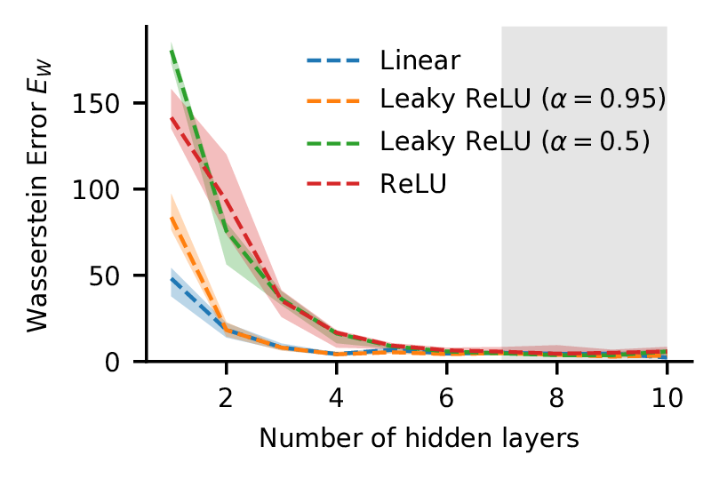
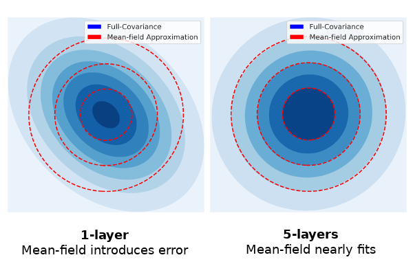
Wasserstein Error. As the network gets deeper, the gap between the full-covariance and mean-field approximation to the true posterior shrinks.

When we use these samples from the true posterior, we can then check how much error the mean-field assumption introduces. One way to assess this looks at Wasserstein distance. We calculate the Wasserstein distance between the mean-field approximation and the true posterior, and also calculate the distance between a full-covariance approximation and the true posterior. The difference between the two of these is a measure of the extra error introduced by using the mean-field assumption (above and beyond the error that comes from using a Gaussian approximation, which is a separate issue).

What we see is that this measure of the error introduced by the mean-field assumption starts large but falls rapidly as the model gets deeper, and by the time you have four or so layers it becomes very small indeed (a bias in the way this is estimated means it will never go to zero). We show here that the behaviour of a ReLU, LeakyReLU with various hyperparameters, and a model with linear ‘activations’ all behave similarly. That will end up being suggestive when we examine the theory later, extending some analysis in the linear case to piecewise non-linear functions.

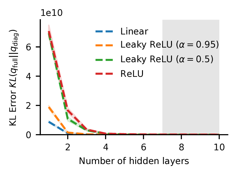
KL Error. As the network gets deeper, the gap between the full-covariance and mean-field approximation to the true posterior shrinks.

Note that we keep the same model size, roughly 1000 parameter, for all of these, tweaking the width as we increase the depth. The experiment uses a simple dataset, scikit-learn’s two moons, so we need to bear that in mind when deciding how much weight to put on this result. The shaded region reflects the area where we start to trust the samples from HMC a little less, based on our diagnostics, but that probably doesn’t affect our conclusions a great deal in any case. There are other details and caveats addressed in the paper.

We have another way of investigating these samples too. If we calculate the Kullback-Leibler divergence—\(KL(q_{full}||q_{diag})\)—it can give us an estimate of the amount of information that we lose by using the mean-field assumption relative to the full-covariance approximate posterior. This tells almost exactly the same story.

What this is hinting to us, is that depth matters to the true posterior. In particular, in deeper neural networks there is at least one mode of the true posterior that is ‘nearly mean-field’ and so the ‘cost’ of the mean field approximation appears to decrease with depth.

Big models: Imagenet

The analysis above looks at fairly small models, but our hypothesis is mostly about very large models. In those large models, it is much harder to get a good sense of how the true posterior behaves. We take a different tack. Let’s look at some comparisons from the literature of different mean-field and structured-covariance approaches on ImageNet.

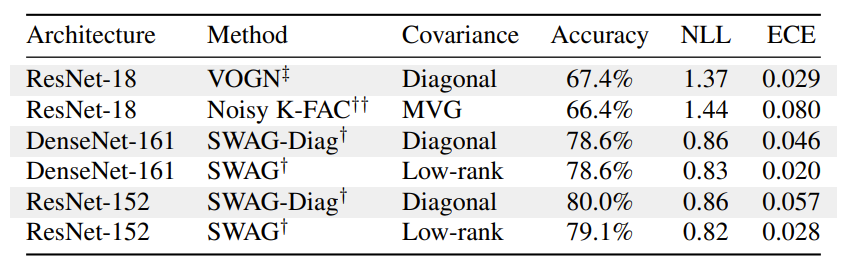
In large networks, structured covariance does not offer a clear advantage in accuracy or uncertainty.

The grey-shaded rows are mean-field (diagonal) methods, while the white-shaded rows are structured approximations using the same neural network architecture. The only clear result is that there isn’t a clear winner. In some cases, the diagonal method has better negative log-likelihood and expected calibration error (measures of aleatoric uncertainty) and sometimes worse. The accuracy seems slightly better for the diagonal approaches. I certainly won’t conclude from this that mean-field is better, but the benefits of adding complexity to the covariance are not apparent. And given that the structured covariance methods take significantly longer to run (~2x longer per epoch for the most efficient versions) and are harder to implement for variational inference, it may not be worth the effort.

Why? Complicated connections can ‘simulate’ complicated distributions.

We’ve reviewed a few suggestive empirical results (more are in the paper). Can we explain these phenomena? In fact, the behaviour may not be that surprising. We start by considering linear models, where it is easy to see that a deep mean-field distribution over weights can result in a distribution over function outputs which has covariance similar to a shallower full-covariance distribution. We even show that the commonly used Matrix Variate Gaussian or K-FAC structured covariance approximation is a special case of three mean-field layers stacked on top of each other with no non-linearities in between.

Then we’ll introduce a new tool, the local product matrix that lets us bridge results from this linear setting into commonly used piecewise-linear neural networks like ones that use Leaky ReLUs.

Last, we’ll consider a different simplifying assumption, looking at the Universal Approximation Theorem in wide neural networks, to see why at least one mode of the true posterior can be approximated by a mean-field network.

Investigating the linear case

Think about a fully-connected neural network without the activation functions. For example, wherever there would have been a ReLU we replace it with the identity. The resulting network is just matrix multiplication. Consider a network with \(L\) layers, each of which has a weight matrix \(W^{(l)}\) for \(1 \leq l < L\). The whole network, with non-linear activations stripped out, is just:

\[\mathbf{y} = \prod^{L}W^{(l)}\mathbf{x} = M^{(L)}\mathbf{x}\]

where we have defined \(M^{(L)}\) as the product matrix.

It’s straightforward to see why the product matrix can have off-diagonal correlations even if each individual weight matrix is mean-field. Let’s zoom in on the simplest case: a two-layer model with 2x2 weight matrices.

\[\begin{aligned}\mathbf{y} &= M^{(2)}\mathbf{x}\\ &= \begin{pmatrix}A_{11} & A_{12}\\ A_{21} & A_{22}\end{pmatrix}\begin{pmatrix}B_{11} & B_{12}\\ B_{21} & B_{22}\end{pmatrix}\mathbf{x}\\ &=\begin{pmatrix}\color{red}{A_{11}}\color{blue}{B_{11}}\color{black} + A_{12}B_{21} & \color{red}{A_{11}}\color{black}B_{12} + A_{12}B_{22}\\ A_{21}\color{blue}{B_{11}}\color{black} + A_{22}B_{21} & A_{21}B_{12} + A_{22}B_{22}\end{pmatrix}\mathbf{x}.\end{aligned}\]

Plainly, elements of the product matrix share terms, and are in general correlated even when the individual elements of the weight matrices are assumed to be diagonal.

In linear models, there’s a straightforward correspondence between the weights and functions. So the deeper mean-field model can express distributions over functions that would require off-diagonal covariance in a shallower model.

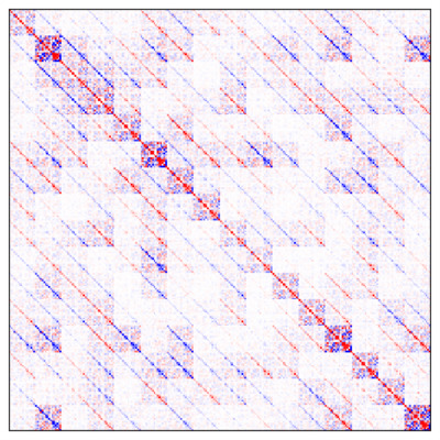
FashionMNIST linear model product matrix covariance. Deep mean-field layers induce a product matrix whose covariance has complicated off-diagonal correlations.

We can see this directly in a trained model. Below, we show the covariance matrix of the product matrix of a deep linear network trained on FashionMNIST. Even though it is composed only of mean-field weight matrices, the product has complex off-diagonal covariance behaviour (here, we show a 10 layer product matrix covariance, estimated with 10,000 samples).

We show two specific mathematical results about this setting, in addition to deriving the explicit form of the weight covariance that you get from the product of multiple mean-field layers.

First, we show that 3+ layers suffice to have non-zero covariance between any and all elements of the product matrix. This starts to suggest how adding depth will let the mean-field layers ‘simulate’ a shallower full-covariance model, where doing so is helpful.

Second, we show that the Matrix Variate Gaussian or K-FAC approximate posterior is a special case of the product of three mean-field layers. That is, in the linear case at least, an MVG approximation does not allow you to represent a function distribution that the linear mean-field would not allow if you overparameterized the linear function.

New tool: local product matrix

So far, we have been considering only linear models. But our experimental results with Hamiltonian Monte Carlo suggest that the dynamics of linear models might not be that different from non-linear ones. We can make this more precise by introducing a local product matrix.

The details are mathematically tricky, and can be found in the paper. But the core idea is that when we use a piecewise-linear activation like a ReLU, although the function as a whole is non-linear, it is composed of many linear functions within different regions of input space. These regions can become extremely small, but they still allow us to construct a random variate, for any given input, which is a local product matrix centred on that input. Because we can describe the product matrix of each individual sample from the weight distribution, we are able to describe the covariance of elements in the local product matrix also.

As a result, we are able to show that the result from above extends to piecewise linear networks also. Three or more layers is enough to allow non-zero covariance between any and all elements of the local product matrix for typical inputs.

Universal Approximations

A final lens looks at the approximation of arbitrarily wide neural networks, which allows us to take advantage of the universal approximation theorem — which states that a neural network with a hidden layer and non-polynomial activation can approximate an arbitrary continuous function arbitrarily closely. We show that a network with three layers of weights can therefore approximate any fixed target distribution, such as the true posterior, arbitrarily closely. The rough construction is that the first weight layer introduces an arbitrary random variable, and the rest of the network uses the universal approximation theorem to transform that random variable onto the target.

What this suggests this that there is at least some mean-field network that expresses a function output distribution that is nearly the same as the true posterior predictive. However, we note that this cannot be taken as showing that variational inference will find this distribution. For that sort of claim, we need to look at empirical results, such as those above.

Conclusion

Researchers have worried that the mean-field approximation is too restrictive. In small networks, we think it probably is. But in larger, deeper, networks, the complexity of the network can substitute for the complexity of the distribution.

As a consequence, we feel the research community should put more emphasis on solving the problems that arise in scaling simple posterior approximations to large models, rather than adding fancy nuance to small models. Big models make it easier to be approximately Bayesian, not harder, and we should take advantage of that.

Acknowledgements

Many people contributed to the work of this paper. We especially want to thank the anonymous reviewers, who were very generous with their time and an enormous help and sadly cannot be personally thanked. In addition, Adam Cobb and Angelos Filos helped with experiments in the paper, while we further benefited from conversations with Wendelin Boehmer, David Burt, Adam Cobb, Gregory Farquhar, Andrew Foong, Raza Habib, Andreas Kirsch, Yingzhen Li, Clare Lyle, Michael Hutchinson, Sebastian Ober, and Hippolyt Ritter.

OATML