OATML

TL;DR: We have released the Shifts benchmark for robustness and uncertainty quantification, along with our accompanying NeurIPS 2021 Challenge! We believe that Shifts, which includes the largest vehicle motion prediction dataset to date, will become the standard large-scale evaluation suite for uncertainty and robustness in machine learning. Check out the challenge website, read our whitepaper, browse our GitHub for baselines and data documentation, and join our Slack channel for discussion!

Dealing with Distributional Shift

The problem of distributional shift — namely, that the test distribution differs from the training distribution — is ever-present in machine learning. This is a serious issue in critical use cases where models have direct impact on human well-being: for example, in finance, medicine, or autonomous vehicles. A model that fails to generalize in such settings might result in dangerous or catastrophic behavior; the failure of a low-level component in an assisted driving system (ADS) to distinguish a trailer from a bright sky led to the first fatality involving an ADS in 2016 [NHTSA, 2017].

The robustness and uncertainty estimation communities have formally taken on the challenge of distributional shift, and made a great deal of progress in recent years [Gal and Ghahramani, 2015, Wen et al., 2018, Wu et al., 2019, Neklyudov et al., 2018, Farquhar et al., 2020, Rudner et al., 2021, among many others]. For example, ensembling [Lakshminarayanan et al., 2017] and sampling-based uncertainty estimates [Gal and Ghahramani, 2016] are commonly used in detecting misclassifications, out-of-distribution inputs, adversarial attacks [Carlini et al., 2019, Smith and Gal 2018], and active learning [Gal et al., 2017, Kirsch et al., 2019].

However, these ensemble and sampling methods are costly, requiring multiple forward passes to obtain high-quality uncertainty estimates. Some cheaper methods in deterministic uncertainty estimation are gaining prevalence [Malinin and Gales, 2018, van Amersfoort et al., 2020, Liu et al., 2020, Malinin et al., 2020], however they still underperform more expensive methods, and some need access to distributionally shifted data at training time.

Benchmarks for Robustness and Uncertainty Quantification

In pursuit of safe and reliable machine learning deployments in the wild, we ought to encourage the development of more efficient and performant uncertainty estimation methods. We believe the best way to do so is through datasets and benchmarks. Major advances in computer vision, natural language, and reinforcement learning are often attributed to the challenging yet easy-to-use benchmarks which have become clear “goalposts” for researchers, such as ImageNet [Deng et al., 2009], GLUE [Wang et al., 2018], and ALE [Bellemare et al., 2013] respectively.

Yet little focus has been directed towards the development of large-scale benchmarks in robustness and uncertainty with real-world distributional shifts. Most are small-scale (e.g., UCI [Dua et al., 2017] regression datasets), or add variations to well-manicured datasets, often in image classification (CIFAR-10/100 [Krizhevsky et al., 2009], ImageNet [Deng et al., 2009, Hendrycks & Dietterich, 2019, Hendrycks et al., 2020, Hendrycks et al., 2021]). Most commonly, these variations are synthetic distributional shifts such as Gaussian blur, which yield examples far from the images we might encounter at deployment (e.g., in ImageNet-C [Hendrycks & Dietterich, 2019], Figure 1).

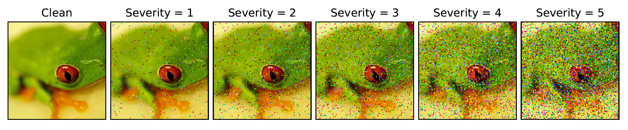
Figure 1: ImageNet-C [Hendrycks & Dietterich, 2019] introduces a variant of ImageNet with synthetic corruptions, such as Gaussian noise with increasing severity.

A couple benchmarks do consider real-world shifts, but focus on more specific problems such as diabetic retinopathy [Filos et al., 2019] or domain adaptation with labels for each setting (e.g., the camera model used to take each picture) [Koh et al., 2020].

Introducing the Shifts Challenge

In collaboration with Yandex Research and the University of Cambridge, we are releasing the Shifts Challenge, a NeurIPS 2021 Competition and open-source benchmark of distributional shifts across three tasks: Weather Prediction, Machine Translation, and Vehicle Motion Prediction.

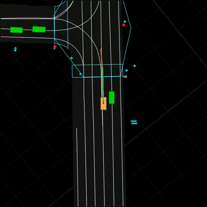
Figure 2: Vehicle Motion Prediction. Given an HD map of the surroundings and positional information on vehicles and pedestrians (collectively, a scene), one must predict the future trajectory of a vehicle.

All three tasks involve new datasets drawn from production settings at Yandex (Yandex.Weather, Yandex.Translate, and Yandex Self-Driving Group respectively). These datasets are large-scale: for example, the Vehicle Motion Prediction dataset is the largest of its kind, with almost 50% more footage than the Waymo Open Dataset [Sun et al., 2019] (see an example of motion prediction in Figure 2). The three tasks span challenging data modalities: Weather Prediction is a tabular task, a domain in which deep learning classically struggles versus tree-based models; Machine Translation is categorical sequence modeling; and, Vehicle Motion Prediction is continuous sequence modeling.

Most importantly, each task considers real-world distributional shifts. In Weather Prediction, models are evaluated on data that occurs later in time than the training data, is distributed differently across world locations, and contains climates unseen at training time (snowy or polar regions). In Machine Translation, we evaluate how models trained on literary text perform in the presence of casual language use from Reddit, for example containing slang and improper grammar. Finally, in Vehicle Motion Prediction, models must perform well in new locations and in the presence of unobserved precipitation (e.g., transfer well from clear days in Moscow to snowy days in Ann Arbor).

For each datapoint in an evaluation dataset, Shifts competitors are expected to produce a prediction along with an accompanying uncertainty measure, which quantifies the extent to which the model is (un-)confident in its prediction. This lack of confidence could reflect encountering an inherently noisy or multimodal datapoint (aleatoric uncertainty) or an unfamiliar situation (epistemic uncertainty). See Kendall and Gal, 2017 for a primer on these two types of uncertainty.

Read on to see how we thought through our evaluation method of choice for the Challenge: retention curves evaluated jointly over in-domain and out-of-domain data.

Designing Metrics with Real-World Distributional Shifts

The major challenge we faced in developing the Shifts Competition was deciding on an appropriate metric to jointly evaluate robustness and uncertainty quantification. Ideally, we would use this single metric to rank model submissions on each of the tasks.

The standard manner of measuring robustness is to simply report a predictive metric evaluated over a distributionally shifted dataset.

Uncertainty quantification is less straightforward in the context of real-world shifts. The common task to evaluate it is out-of-distribution (OOD) detection, in which in addition to a prediction for each example, we also produce a per-example uncertainty value. This value could be obtained through a statistic of the likelihood, or the disagreement amongst samples from the predictive distribution or ensemble members, for example. We then use this uncertainty value to flag each example as in- or out-of-domain. However, standard OOD detection falls short in uncertainty quantification for real-world shifts. We’ll illustrate this with two situations, drawing examples from location-based shifts in Vehicle Motion Prediction.

Situation 1 (Figure 3): there could be datapoints in-domain which come from a rare subpopulation and on which the model gets high error. In this example, both the training and the test data are from Moscow (in-domain). Suppose a tiny proportion of Moscow scenes have extremely dense traffic. If error is high on those datapoints, uncertainty should also be high, even if the datapoints are technically in-domain because they are collected from the same city as the training data.

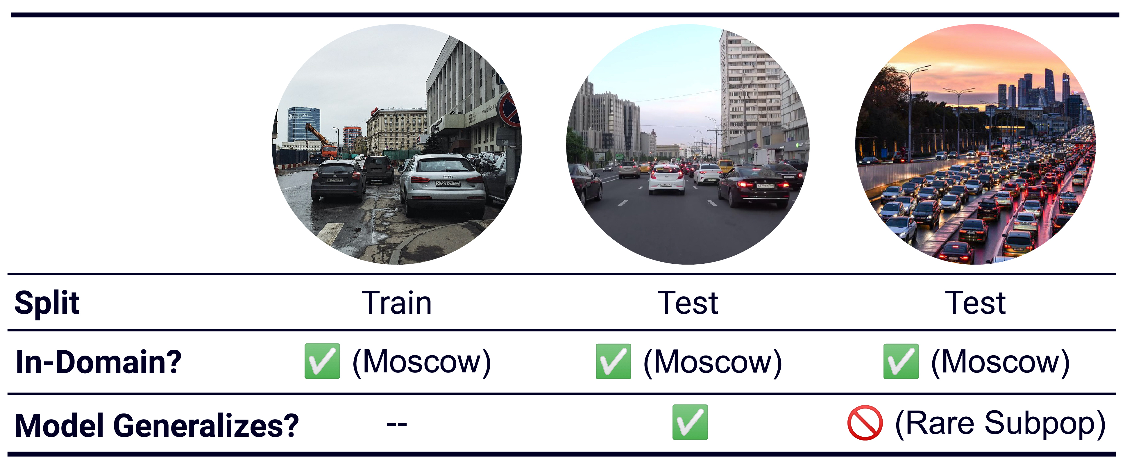
Figure 3: Even when we evaluate on in-domain Moscow motion prediction data, we may encounter examples from a rare subpopulation on which the model performs poorly. This high error should be reflected with high uncertainty.

Scenario 2 (Figure 4): there could be datapoints in the distributionally shifted dataset on which the model nevertheless generalizes well and achieves low error. For example, when training on Moscow and testing on the distributionally shifted Tel Aviv dataset, there may still be a subpopulation of familiar scenes at test time. In other words, a chosen shift may encompass many meaningful changes in aggregate over the dataset — road geometry, traffic laws, driver etiquette, etc. — but there still may be particular datapoints in the shifted dataset that are highly similar to the training data.

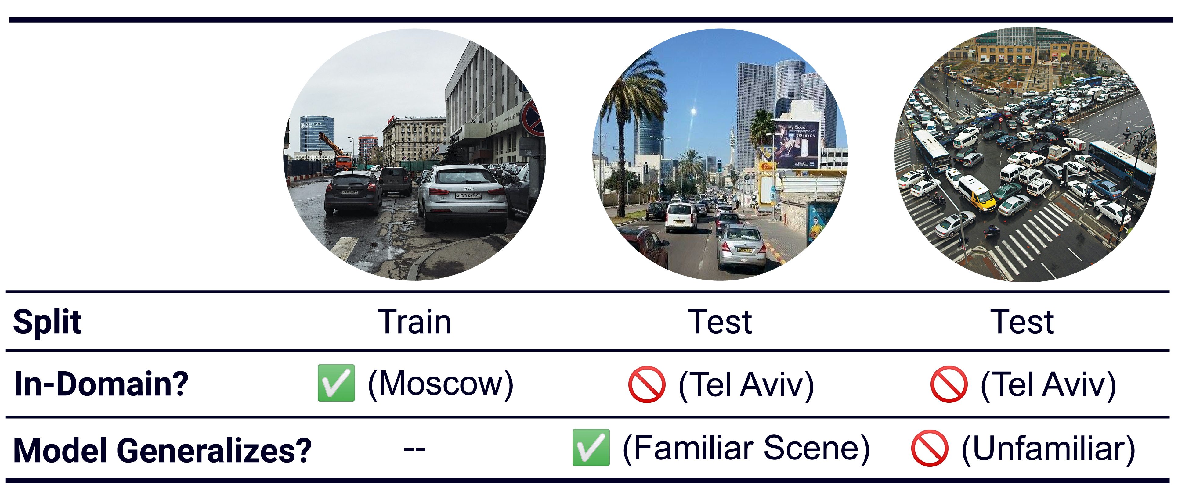
Figure 4: When training on Moscow scenes and evaluating on distributionally shifted Tel Aviv scenes, we may still encounter test examples that are similar to those from Moscow. High performance on such scenes should be reflected with low uncertainty.

To summarize, some in-domain examples might still be unexpected and hence challenging for the model, and some distributionally shifted examples might be familiar and hence easy for the model. Therefore, standard OOD detection is an inappropriate metric for the quality of uncertainty on real-world distributional shifts.

What is Good Uncertainty?

So what might be a better way to determine what is “good” uncertainty? Preferably, one compatible with our desire to use complex, real-world data?

One desideratum for uncertainty is that it ought to correspond with error. As an example is increasingly “shifted” in some respect, we would expect a model to do more poorly on it, i.e., have increasing error. This should be reflected with increasing uncertainty.

Second, our uncertainty estimates should be useful in avoiding dangerous or catastrophic situations. For example, in our self-driving setting (Figure 5), when the model encounters an ambiguous or unfamiliar setting, it should assign that scene with a high uncertainty, and perhaps even give control back to the human passenger [Filos et al. 2020].

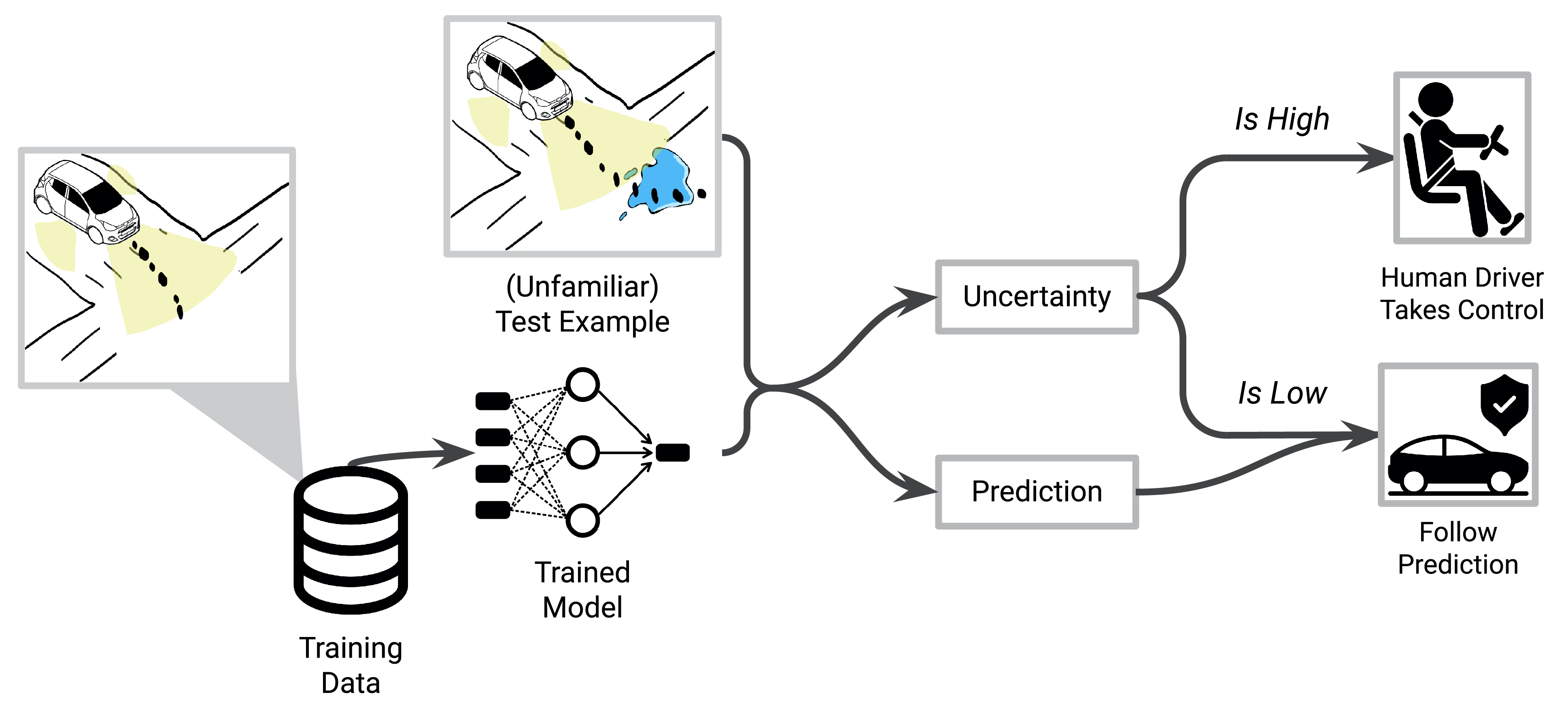
Figure 5: Uncertainty estimates should be usable in human-in-the-loop systems. For example, when an assisted driving system encounters an unfamiliar or challenging environment, it can yield control of the vehicle to the human passenger.

We might see a similar setup in a clinical setting, in which a model diagnosing whether or not a disease is present should report high uncertainty in the same circumstances, and refer that patient to a specialist.

A Primer on Retention Curves

This brings us to our metric of choice in the Shifts Challenge. We jointly evaluate robustness and uncertainty quantification with retention curves over in-domain and shifted data. Here’s an example of retention curves for some different models (Figure 6).

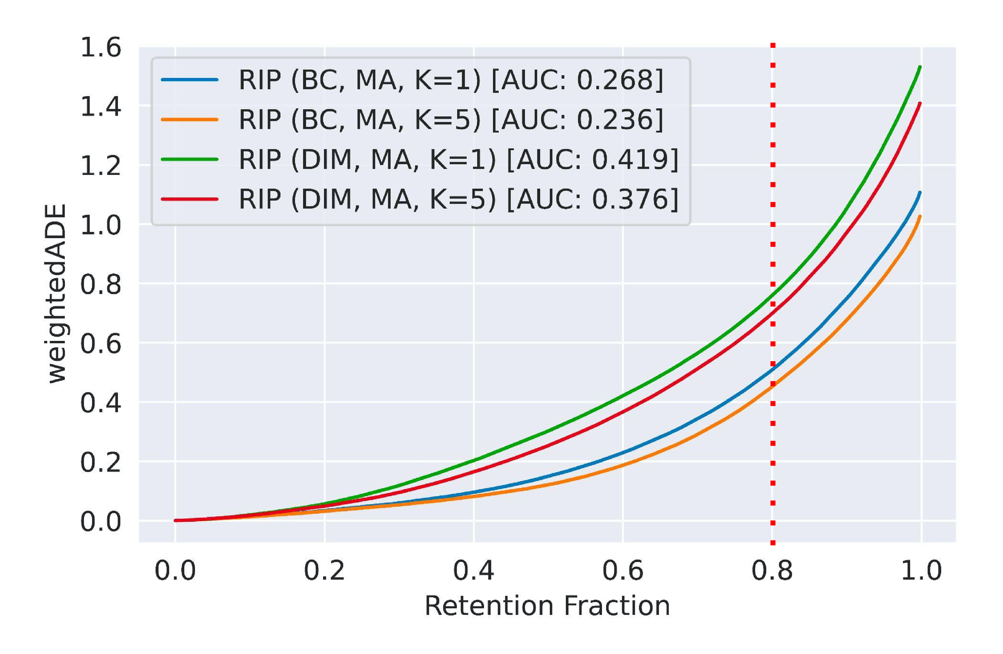
Figure 6: The retention curves of four motion prediction models, defined with respect to a Shifts metric (weightedADE). Because a lower ADE is better, a smaller AUC is better.

A retention curve is always defined with respect to some domain-specific metric of predictive performance. In this case we have a variant of Average Displacement Error (ADE), an MSE-like metric commonly used for motion prediction, on the y-axis (see our whitepaper for a full description of all metrics across the three tasks).

On the x-axis, we see the retention fraction. This means that, for example, at retention fraction 0.8 (red dotted line), the model is allowed to “defer” 20% of all datapoints to a human labeler. The other 80% are retained. Naturally, we will defer the 20% of datapoints with the highest uncertainty values. And so on, we sweep over all possible retention fractions, and finally we report the area under the retention curve. Because a lower ADE is better, we want to minimize the area under the curve.

Retention Curves Capture Robustness and Uncertainty Quantification

Retention curves capture both standard notions of robustness and of uncertainty.

We could improve our area under the curve simply by improving predictive performance, i.e., robustness when we only consider performance on shifted data.

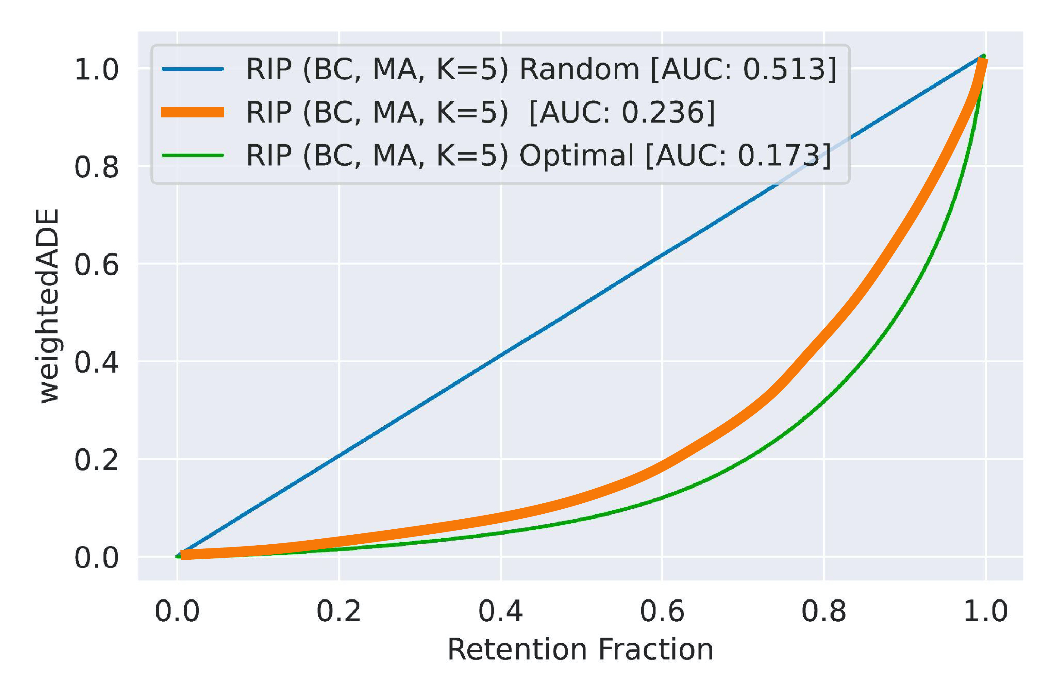
Figure 7: Retention curve of a Vehicle Motion Prediction model, RIP (BC, MA, K=5), in orange. We also illustrate performance with best- and worst-case uncertainty estimates (in green and blue respectively).

Alternatively, we could keep our predictions exactly the same (meaning our errors are the same for each example), but improve the area under the retention curve with improved uncertainty estimates.

In Figure 7 we see a retention curve for a baseline method in orange. The blue plot traces the retention curve assuming random uncertainty values, i.e., they are uninformative and the model isn’t able to properly defer difficult examples. On the other hand, in green we see the optimal curve, where the uncertainty values are perfectly correlated with the error, and the examples which give the model the most trouble are the first to go.

Retention curves are a natural way to jointly evaluate robustness and uncertainty for real-world distributional shifts. We prominently featured the Vehicle Motion Prediction dataset in our examples above, but note that we use retention curves on the other datasets with domain-specific performance metrics (e.g., MSE for regression in Weather Prediction, GLEU for Machine Translation).

Conclusion and Competition Timeline

The Shifts Challenge introduces three new datasets drawn from production settings: Weather Prediction, Machine Translation, and Vehicle Motion Prediction. Shifts covers a variety of challenging and unique domains including tabular data and sequence modeling. We provide canonical partitions of the data which include evaluation subsets either matched to or distributionally shifted from the training distribution.

Each of the three datasets is accompanied by a challenge track, and each track is split into two stages: development and evaluation.

In the development stage (July - early October 2021) participants are provided with training and development data which they use to create and assess their models. We provide a development leaderboard for each track, which participants can use to follow their progress and compare their models.

In the evaluation stage (October 17 - 31, 2021), participants are provided with a new evaluation dataset which contains examples that match the training data, as well as examples that are mismatched to both the training data and the development data from the previous stage. During this period, participants will adjust and fine-tune their models, with the final deadline for submission on October 31. At the end of the evaluation phase, the top scoring participants will present their solutions to the competition organizers.

Organizers will verify that models comply with competition rules during November with competition results announced November 30, 2021. Evaluation dataset ground truth values and metadata will also be released at this point.

We hope for Shifts to become a default testbed for new methods in robustness and uncertainty. Register for the Shifts NeurIPS 2021 Competition at the challenge website, check out a discussion of our data, metrics, and baselines in our whitepaper and their implementation at our Github, and please feel free to reach out to us with questions in our Slack channel.

Best of luck to the competitors!

Acknowledgements

The Shifts Challenge is a joint collaboration between the Oxford Applied and Theoretical Machine Learning Group, Yandex Research, and the University of Cambridge. OATML work was sponsored by:

More blog posts here: OATML Blog