Itô and Stratonovich; a guide for the perplexed

The Itô & Stratonovich integrals
This post is based on one that was, for a long time, hosted on my personal website. I recieved a relatively large amount of communication about it, and I so I think that it seems to have been popular and useful. I’m now getting close to graduation, and I thought it would be good to move it somewhere more permanent so that it doesn’t get lost to time.
I originally wrote this post around 2018 - since then, if anything, SDE’s have become even more important in machine learning with the recent popularity of diffusion models, and progress on learning parameterised SDEs so I feel that this overview remains at least as relevant for ML researchers as it was then, though this post is about the underlying maths than anything ML specific.
Something many people, including myself, find quite confusing when learning about SDE’s is the existence of two formulations of the stochastic calculus; the Itô and Stratonovich formulations. When I first read about it, it seemed like there were two mathematical treatments of the same physical process that give different answers. As we will hopefully see, this isn’t actually a very accurate description, but it’s the impression you can still get from a lot of textbooks and writing on the subject. SDEs require some fairly heavy duty mathematics, and most of the work I was able to find on them wasn’t massively accessible, and tends to focus on technical details over intuition. This article is designed to be as concise and simple a statement as possible of the origins of the two formulations, how they are related, and whether the difference really matters1. I’ve tried to avoid going into the measure-theoretic treatment and more technical proofs in favour of a high-level, intuitive overview that is still morally correct. There is a list of references if you want to get deeper into the details of the ideas I’m going over here.
This is a summary and overview, not original work. Most derivations etc. are based on those in the references; any mistakes are my own.
The problem
The basic problem addressed by SDEs is how to deal with noise in a physical process. That is, we have a system described by a standard differential equation
\[\begin{aligned} \frac{dx}{dt} = f(x,t)\end{aligned}\]and we want to extend this model to deal with the presence of intrinsic noise. Note that we are not talking about observation noise; the noise effects the evolution of the state \(x\). Lets call the noise term (a random variable) \(\xi_t\) and we can imagine an equation that looks something like this;
\[\begin{aligned} \frac{dX}{dt} = f(X,t) + \text{“}\sigma(X,t) \xi_t\text{''}\end{aligned}\]where \(\sigma(x,t)\) is a deterministic function determining how the noise process \(\xi_t\) affects the state. In this way, we can keep \(\xi_t\) as a generic noise term. The reason for the quotation marks will become clear.
Of course, the deterministic equation has the general integral solution
\[\begin{aligned} x(T) = x(0) + \int_{t=0}^{T} f(x, t)dt\end{aligned}\]and so we expect it’s stochastic counterpart will have solution that looks something like this
\[\begin{aligned} X(T) = X(0) + \int_{t=0}^{T} f(X, t)dt + \text{“} \int_{t=0}^{T} \sigma(X,t) \xi_t dt \text{"}\end{aligned}\]requiring us to somehow integrate over the noise process. The question, then, is how we assign meaning to the terms in quotation marks. We should probably start by choosing some specific random process for the noise term \(\xi_t\). We want it to have the following properties, approximately like that of normally distributed noise for discrete observations;
-
The noise is zero mean: \(\mathbb{E}[\xi_t] = 0\) for all \(t\).
-
The noise is uncorrelated: for any \(t,t'\) such that \(t \ne t'\), \(\mathbb{E}[\xi_t\xi_{t'}] = 0\)
-
The noise is stationary: for any set of times \(t_1, t_2,...t_n\), the joint distribution \(P(\xi_{t_1}, \xi_{t_2} ...)\) is the same as \(P(\xi_{t+t_1}, \xi_{t+t_2} ...)\) for any \(t\).
The reason we want the first condition is pretty obvious; if the noise had a non zero mean, then it would produce a drift over time, and we would rather treat the drift as part of the deterministic function \(f\). Similarly, if the noise was non-stationary, we could absorb that into the function \(\sigma\); we want a ‘standard’ noise term. These conditions describe white noise, a random signal with no characteristic frequency.
This seems reasonable enough, and fairly well motivated by the noise one encounters in real systems (for example, TV static). However, continuous time white noise is actually quite a bizarre and poorly behaved mathematical object. It turns out to be impossible to construct a white noise process \(\xi_t\) which also has continuous paths, which seems like an important feature for defining well behaved differential equations. Indeed, a true white noise signal would have a completely flat Fourier spectrum, which would imply that it had infinite energy 2. So we cannot give the equation a sensible meaning by setting \(\xi_t\) to a random process directly.
We need a different way, then, to interpret the noise term, if we are going to end up with a sensible mathematical model for noisy dynamics. One way to arrive at a more meaningful result is to anticipate the fact that we want to define a stochastic integral, and so split \(T\) into \(N\) discrete intervals and consider the discrete equation
\[\begin{aligned} X_T = X_0 + \sum_{t=1}^{N} f(t, X_t) \Delta t + \sum_{t=1}^{N} \sigma(t, X_t) \Delta W_t\end{aligned}\]where \(\Delta W_t = W_{t+1} - W_{t}\) are the increments of some random process \(W_t\). Now, our assumptions imply that we would like the process to have stationary, independent increments with zero mean. It turns out there is only one such process with continuous paths: Brownian motion, also known as the Wiener process, which is a continuous time generalisation of a random walk.
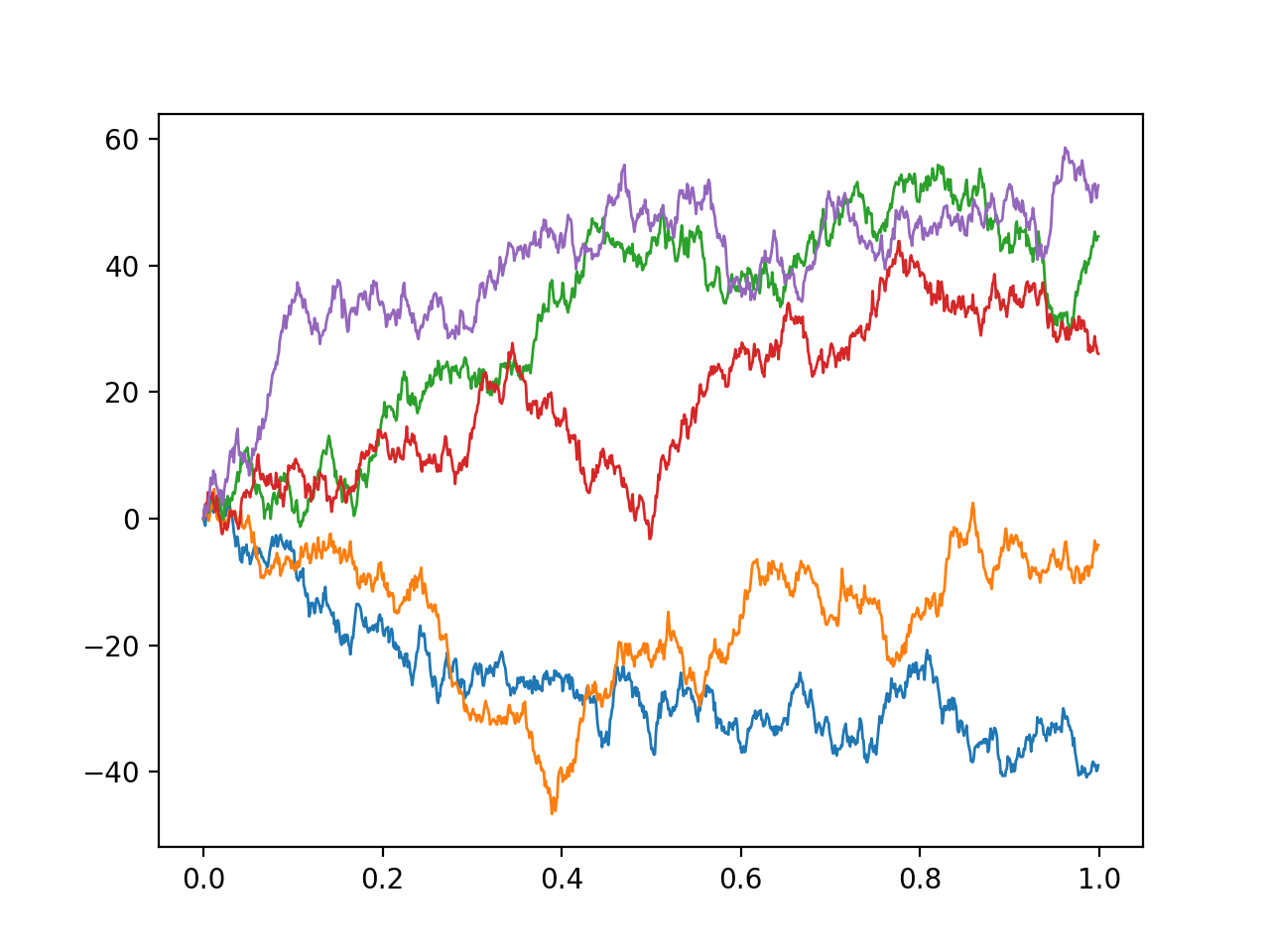
Sampled paths of brownian motion
The Wiener process can be thought of as the integral of white noise. It is differentiable nowhere; its derivative would be the white noise process discussed above. Brownian motion \(B_t\) is an example of a Gaussian process; for any finite collection of times \(t_1, t_2, ... t_n\), the joint distribution of \(B_{t_1}, B_{t_2}...\) is a multivariate Gaussian, with mean zero (for Brownian motion starting at zero) and a covariance matrix \(\Sigma\) whose entries are given by
\[\begin{aligned} \Sigma_{ij} = \mathbb{E}[B_{t_i} B_{t_j}] = \min(t_i, t_j)\end{aligned}\]For brevity here, I’m going to mostly take the above as a sensible definition without going much into physical motivations, but Brownian motion has many physical applications, with the original one being the motion of a particle suspended in a fluid. The basic physical intuition behind the idea that \(B_t\) is an integral of white noise is that in an interval \(\Delta t\), our particle gets hit by a large number of uncorrelated kicks in random directions with bounded variance, which will lead to a Gaussian change of momentum in that interval.
It follows directly from the above definition that Brownian motion has independent increments; if \(t_1 < t_2 < t_3 ...\), then
\[\begin{aligned} \mathbb{E}[(B_{t_{i+1}} - B_{t_i}) (B_{t_{j+1}} - B_{t_{j}})] &= \min(t_{i+1},t_{j+1}) - \min(t_{i+1},t_j) - \min(t_i, t_{j+1}) + \min(t_{i}, t_{j}) \\ &= t_{i+1} - t_{i+1} - t_{i} + t_{i} \;\;\;\text{when}\;\; t_i < t_j \\ &= 0\end{aligned}\]and the variance of increments is
\[\begin{aligned} \mathbb{E}[(B_{t} - B_{t'})^2] &= \mathbb{E}[B_{t}^2] + \mathbb{E}[B_{t'}^2] - 2\mathbb{E}[B_{t}B_{t'}] \\ &= t + t' - 2 \min(t,t') \\ &= |t-t'|\end{aligned}\]Brownian motion is the only process with continuous paths that satisfies our list of criteria, so we will use as our discrete model
\[\begin{aligned} X_{k+1} - X_{k} = f(t, X_t) \Delta t + \sigma(t, X_t) \Delta B_t \\ X_T = X_0 + \sum_{t=1}^{N} f(t, X_t) \Delta t + \sum_{t=1}^{N} \sigma(t, X_t) \Delta B_t\end{aligned}\]in integral or derivative form. We can now try to get back to a continuous time model by taking the limit as we divide the interval into smaller and smaller pieces (\(N \to \infty\)).
The stochastic integral
Let’s quickly recall how the standard (Riemann) integral can be defined. We have some function \(f(t)\) we want to integrate over the range \(0,T\). First, we partition the interval into \(t_0,t_1, t_2, t_3,...\), and consider
\[\begin{aligned} \int_0^{T} f(t) dt = \lim_{N \to \infty} \sum_{k=0}^{N-1} f(\hat{t}_k) \Delta t_k,\;\Delta t_k = t_{k+1} - t_k\end{aligned}\]where the width of each interval is \(T / N\), and for each interval \(\Delta t_k\), we choose a value \(\hat{t}_k \in [t_{k}, t_{k+1}]\) at which we evaluate the function. Basically, we replace the function with a series of rectangles, whose heights are \(f(\hat{t}_k)\) and whose widths are \(\Delta t_k\). Since we know how to calculate the area of these rectangles, we can then define the integral as the limit of the sum of the area of the rectangles as we make this approximation tighter and tighter.
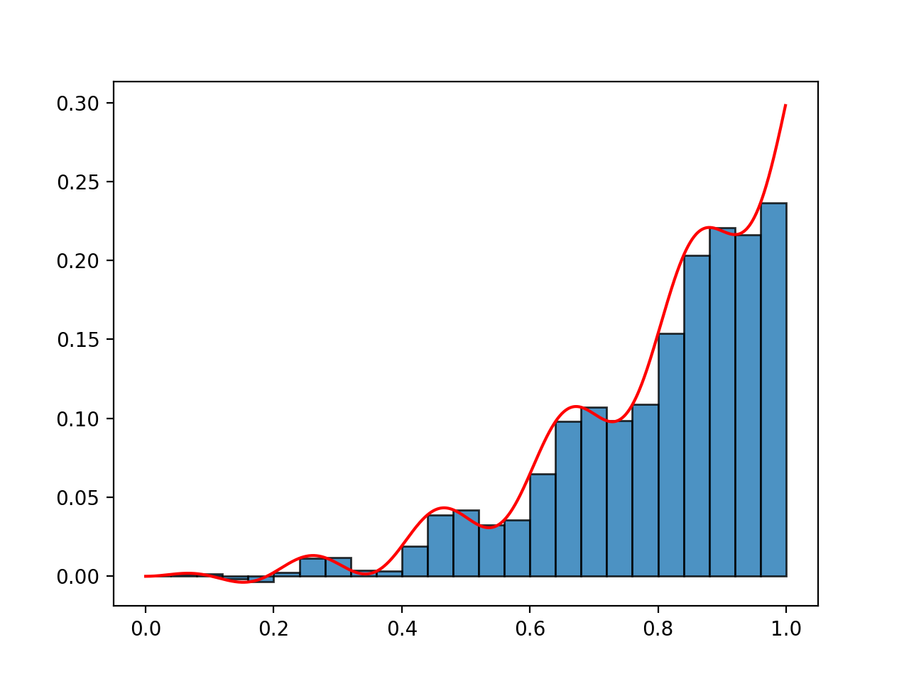
The Riemann integral construction; divide the function up into rectangles. Here, I've evaluated the function at the left edge of each rectangle.
For ordinary, smooth functions, of course, this integral converges to the same value no matter where we choose our rectangle heights \(\hat{t}_k\) in the interval. However, Brownian motion is less well behaved.
To be slightly more precise, the rectangular construction can be thought of as approximating \(f\) as a ‘simple function’, where simple functions are defined in the following way. Let \(\mathbf{1}\) be the characteristic function of a set \(A\); that is \(\mathbf{1}_A(x) = 1\) if \(x \in A\) and \(0\) otherwise. Then, the rectangular construction is the same as a approximating \(f\) with a function of the form
\[\begin{aligned} f(t) \simeq \phi(t) = \sum_k \hat{f}_k \mathbf{1}_{[t_{k}, t_{k+1})}(t)\end{aligned}\]where the \(\hat{f}\) are constants, chosen at some point in the interval as above. For these functions, the area under the curve can be computed very easily as a sum of rectangles. As we take the limit of the intervals becoming infinitesimally wide, the approximation to the function becomes exact and the sum converges to the value of the integral 3
The obvious thing to do next is to try to extend the same idea to random processes. That is, we can consider functions of the form
\[\begin{aligned} \phi(t) = \sum_k \hat{e}_k \mathbf{1}_{[t_{k}, t_{k+1})}(t)\end{aligned}\]for which, following the sum model for SDE’s above, the integral can be defined in terms of discrete intervals in a straightforward way as
\[\begin{aligned} \int_0^{T} \phi(t) dB_t = \sum_k \hat{e}_k \Delta B_k\end{aligned}\]Note that here, the coefficients \(\hat{e}_k\) are not constants, as in the construction for deterministic functions, but random variables, as we are allowed to integrate functions \(\sigma\) which depend on \(X_t\), which is also a random variable.4 It doesn’t have the same geometrically intuitive nature as the Riemann integral, but there is an analogy here; instead of a finite sum of simple functions which are rectangles, we are now dealing with a finite sum of ‘simple random variables’ multiplied by independent increments of a Brownian walk, which are Gaussian. These \(\hat{e}_k\) are analagous to the function evaluations \(\hat f_k\) in the Riemann construction, so in a minute we will think of them as sampling a continuous-time random process at a particular point in time.
And we can try to proceed in the same way; having defined a class of functions whose integral is obvious, analogous to the rectangles of the Riemann construction, we can then consider approximating the functions we wish to integrate as these simple functions, then letting the size of the interval tend to zero.
However, we will run into difficulties immediately. Unlike for continuous functions, whose sum converges wherever we choose the midpoints \(\hat{f}_k\), we will see that we can get very different results depending on where we evaluate the integrated function in the random case. Let the evaluation point be \(\tau_k \in [t_k, t_{k+1})\), and consider integrating \(B_t\) in this way, so \(\hat{e}_k = B_{\tau_k}\). Then, if we consider the expectation, we have
\[\begin{aligned} \mathbb{E} \left[ \int_0^{T} B_t dB_t \right ] &= \mathbb{E}\left[ \sum_k B_{\tau_k} \Delta B_k \right]\\ &= \sum_k \mathbb{E}\left[ B_{\tau_k} (B_{t_{k+1}} - B_{k}) \right] \\ &= \sum_k \min(t_{k+1}, \tau_k) - \min(t_{k}, \tau_k) \\ &= \sum_k (\tau_k - t_{k})\end{aligned}\]but this can be anything between 0 (for \(\tau_k = t_k\)) and \(T\) (for \(\tau_k = t_{k+1}\))! So without a choice of \(\tau\), we are still unable to define the integral of a fairly simple stochastic process without ambiguity. In the above, we didn’t bother writing that we were considering a limit, but it clearly doesn’t affect the argument, as the different answers have no dependence on \(N\).
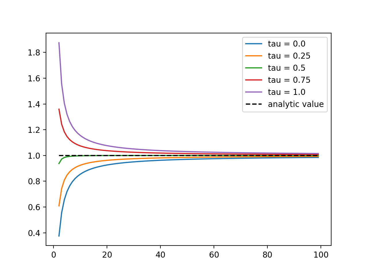
The convergence of the Riemann integral for a simple polynomial with the number of subdivisions of the interval, for various choices of evaluation point. For the Riemann integral, this choice doesn't matter; they all converge quickly to the true value of the integral. This is not always the case for stochastic integrals.
We can fix this problem by simply making a choice, and so we define the integral to be the limit as evaluated for a choice of \(\tau\). The Itô rule says to evaluate the integrand at the left endpoint, corresponding to \(\tau_k=t_k\), while the Stratonovich rule says to evaluate at the midpoint, corresponding to \(\tau_k = \frac{1}{2}(t_{k+1} + t_{k})\). We could, in principle, choose \(\tau_k = \lambda t_{k} + (1 - \lambda) t_{k+1}\) for any value \(\lambda \in [0,1]\), leading to an infinite number of possible versions of stochastic calculus, but these two choices turn out to be the most natural and convenient ones.
Itô or Stratonovich?
The obvious question is which interpretation is the right one?. After all, we just saw that the equations give different answers. If we let
\[\begin{aligned} \int_0^{T} b(x,t) dB_t\end{aligned}\]denote the Itô integral and
\[\begin{aligned} \int_0^{T} b(x,t) \circ dB_t\end{aligned}\]denote Stratonovich’s, then we have two options to interpret our original prototype of a stochastic differential equation. Itô says
\[\begin{aligned} X(T) = X(0) + \int_{t=0}^{T} f(X, t)dt + \int_{t=0}^{T} \sigma(X,t) dB_t\end{aligned}\]and Stratonovich says \(\begin{aligned} X(T) = X(0) + \int_{t=0}^{T} f(X, t)dt + \int_{t=0}^{T} \sigma(X,t) \circ dB_t\end{aligned}\)
and these describe different processes, as we have just seen, since they evaluate the integrals with respect to \(dB_t\) differently. Surely one must be “better?". Lets briefly look at the properties of the two integrals before we return to this question.
Itô
The biggest advantage of Itô’s formulation is that the evaluations of the function are totally uncorrelated with the increment, by construction. That is to say, that because we evaluate the function \(f(x, B_t, t)\) at the left point of the midpoint, our limiting sum is
\[\begin{aligned} \int f(x, B_t, t) dBt = \lim_{N \to \infty} \sum_k f(x_{t_k}, B_{t_k}, t_k) (B_{t_{k+1}} - B_{t_k})\end{aligned}\]But because the increment \((B_{t_{k+1}} - B_{t_k})\) is uncorrelated with \(B_{t_k}\), it’s also uncorrelated with any function of \(B_{t_k}\), and so this always has mean zero.
This leads to the nice property that an Itô integral \(\begin{aligned} \int_S^{T} f(x,t) dB_t \end{aligned}\)
always has mean zero, and is a martingale. A stochastic process \(M_t\) is a martingale if its mean is bounded, and the conditional expectation given access to it’s history up to time \(t'\) is equal to the value at that time; that is
\[\begin{aligned} \mathbb{E}[|M_t|] < \infty \\ \mathbb{E}[M_t | \{M_s, s \le t'\} ] = M_{t'},\;\;\text{for all}\;t' \le t\end{aligned}\]In less formal language, this means that the “best guess" for the future value of a martingale is always the most recent observed value; knowing \(M_{t'}\) is just as good as knowing the entire history of \(M_t\) up to \(t'\). The origins of the term “martingale" are historical; they have been extensively mathematically analysed in the context of gambling5. If \(W_t\) is your wealth at the \(t^{th}\) round of a fair game, like betting on a coin flip, then \(W_t\) is a martingale; on average you end up with the same amount of money you started with.
It is slightly difficult to give a non-technical overview, but this property turns out to be very convenient mathematically, due to some nice theoretical properties of martingales. For instance, one can make use of the martingale property when computing the conditional expectation of an Itô process. In general, it is easier to analyse and prove theorems about the Itô integral for this reason.
The choice of the function evaluation “before” the observation of noise also seems natural if you think of a stochastic process as being the limit of a discrete one as the time-per-round becomes infinitesimal, as we used above to derive an SDE. Obviously, in a discrete-time decision process, you have to make your decision before you observe new information, and the Itô integral makes the current function value statistically independent of the current noise increment, which reflects this. 6
On the other hand, the Itô integral leads to a modification of the chain rule of calculus for changing variables. If we have an Itô process \(\begin{aligned} dX_t = f(X_t,t) dt +\sigma(X_t, t) dBt \end{aligned}\)
and we want the equation of a new random process \(Y_t\), where \(Y_t = g(t,X_t)\), and \(g\) is a twice differentiable function, the Itô SDE for \(Y_t\) is given by
\[\begin{aligned} dY_t = \frac{\partial g}{\partial t}(t, X_t) dt + \frac{\partial g}{\partial x}(t, X_t) dX_t + \frac{1}{2}\frac{\partial^2 g}{\partial x^2}(t, X_t) \sigma(X_t, t)^2 dt\end{aligned}\]– Itô’s famous lemma. Here, we have an additional second order term in the noise added to the standard chain rule. I won’t go through a full derivation of Itô’s lemma here, but I will provide a brief, hand-wavey explanation. From the properties of Brownian motion, we can see that
\[\begin{aligned} \mathbb{E}[\Delta B_k ^2] = \Delta t_k\end{aligned}\]which implies that, as we take the limit
\[\begin{aligned} (dB_t)^2 = dt\end{aligned}\]The infinitesimal of \(dY_t\) is given by it’s Taylor expansion; \(\begin{aligned} dY_t &= \frac{\partial g}{\partial t} dt + \frac{\partial g}{\partial x}dX_t + \frac{1}{2}\frac{\partial g^2}{\partial x^2} (dX_t)^2 + ... \\\end{aligned}\)
Normally, we only need to care about the first order Taylor expansion in the infinitessimal limit, but here the second order term in \(X_t\) is relevant because
\[\begin{aligned} (dX_t)^2 = f ^2 (dt)^2 + 2 f \sigma dt dB_t + \sigma^2 (dB_t)^2\end{aligned}\]In the infinitesimal limit, \(dt^2\) and \(dt dB_t\) become negligible faster than \(dt\) and \(dB_t\), but as we saw above, \((dB_t)^2\) is of the same order as \(dt\) and tends to \(dt\) in probability, so we can’t neglect this term. Since the Itô choice means that \(\Delta B_k\) is independent of \(f_k\) and \(\sigma_k\), this leads to the rule \(dt^2 = dt dB_t = 0, dB_t^2 = dt\), from which we get the last term in Itô’s lemma.
Stratonovich
Itô’s lemma is a neat piece of mathematics, but it’s also quite awkward to work with. Stratonovich’s choice avoids this; his choice of evaluation point preserves the standard chain rule, but in the process necessarily gives up the useful martingale properties of the Itô integral.
I mentioned that Itô has a certain intuitive appeal if you think of a stochastic equation as the limit of a discrete time process. Similarly, the Stratonovich integral has a nice physical motivation. Recall, originally, one of the desired properties of white noise \(\xi\) that we wanted was total independence w.r.t time \(\begin{aligned} \mathbb{E}[\xi_t \xi_{t'}] = 0,\;t \ne t\end{aligned}\)
which prevents you from constructing a noise process with continuous paths, and leads to the absurd requirement that we have a signal with a flat power spectrum for all frequencies. The white noise condition above says that for any \(\epsilon\), \(\xi_t\) and \(\xi_{t+\epsilon}\) are totally statistically independent. A more realistic version of this condition is that the characteristic time scale of correlation is finite, but very small, at least compared to the time scale on which we are measuring the system. For example, consider the noise induced in a small object suspended in a fluid, the canonical example of a physical random walk. It’s obvious that while the kicks from particle collisions happen on a much smaller timescale that the macro motion of the particle, they will have some finite, though tiny, correlation time since the particles in the fluid move at finite speed.
If we allow our noise process to have some finite length-scale \(\tau\), then we can draw a process with continuous paths. To be concrete, consider the squared-exponential process, a Gaussian process with covariance
\[\begin{aligned} \Sigma_{ij} = \exp \left[ \frac{-|t_i - t_j|^2}{\tau^2} \right]\end{aligned}\]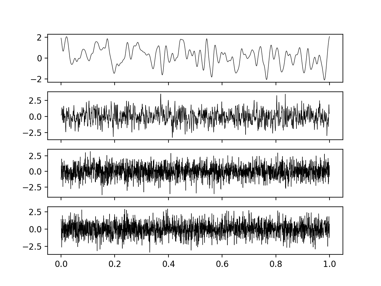
The first three figures are draws from a Gaussian process with a finite correlation length, with this length being decreased gradually. These have smooth, continuous paths. The bottom panel shows a draw from true white noise. As the length scale decreases, the finite correlation noise becomes increasingly similar to white noise, so we can think of white noise as an idealised limit of a series of smooth, continuous processes with increasingly small correlation time.
Clearly, as \(\tau \to 0\), this approaches the idealised white noise process \(\xi\), as can be seen in the figure above. We can therefore consider having some process \(B^\tau_t\), such that as \(B^{\tau}_t \to B_t\) as \(\tau \to 0\), and consider what the process
\[\begin{aligned} \frac{dX_t^\tau}{dt} = f + \sigma \frac{dB^\tau_t}{dt}\end{aligned}\]converges towards. Making this statement more rigorous requires going back to measure theory, and considering the equation that is conditioned on an element of the event space \(\Omega\), that is \(B_t^\tau(\omega)\). This equation is then a standard ODE for all \(\tau\), since \(B_t^\tau(\omega)\) are deterministic, continous functions, and one can show that the \(X^\tau_t(\omega)\) converges to \(X_t(\omega)\) for almost all \(\omega\). More intuitively, we can imagine that the unknown ODE input \(B^\tau_t\) is picked ahead of time, meaning that the system is just a normal ODE with an unobservable state component. These are random ODE’s in the sense that they have an unknown input, but their mathematical behaviour is the same as standard ODEs. It turns out that the solution to these equations converges to the Stratonovich equation
\[\begin{aligned} dX_t = f dt + \sigma \circ dB_t\end{aligned}\]in the limit of white noise (\(\tau \to 0\)). So the physical interpretation of the Stratonovich process is as the limit of a continous time process with coloured noise. Intuitively, this is why Stratonovich preserves the normal chain rule; because we define it as the limit of a series of ODEs, which obviously obey the standard chain rule. However, Stratonovich integrals are not Martingales - with the evaluation of \(f\) at the midpoint of the interval, \(f\) and \(\Delta B_t\) are no longer independent by construction. Intuitively, this is because for a process with finite correlation time, the current value of the process is correlated with it’s value in the future, meaning that we don’t have the nice independence between the current value and the increment we get from the Itô formulation.
Does it matter?
I’ve tried to give an idea of the “philosophical” justification for the approaches taken by the two formulations. To an extent, the popularity of the two reflects this; the Itô integral is more popular in mathematics and finance, where the interpretation as the limit of a discrete steps is somewhat appealing, and (more importantly) the martingale property is convenient. Stratonovich’s rule is more popular in physics, where the limit of smooth noise argument is more compelling. However, it’s easy to exaggerate the importance of this. In particular, the two are mathematically equivalent in the following sense; any Stratonovich process
\[\begin{aligned} dX_t = f(X_t,t) dt + \sigma(X_t, t) \circ dB_t \end{aligned}\]has an equivalent Itô process with identical solutions, which is given by
\[\begin{aligned} dX_t = f(X_t,t) dt + \sigma(X_t, t) dB_t + \frac{1}{2} \frac{\partial \sigma}{\partial x}(X_t, t) \sigma(X_t, t) dt\end{aligned}\]This formula holds in both directions. So if we already have a well defined SDE, either in the Itô or Stratonovich sense, then we can convert between the two conventions arbitrarily, depending on which properties we feel are more convenient for the problem at hand. Notice that the conversion formula basically comes down to a modification of the drift (\(dt\)) term.
The only time ‘interpretation’ comes into it is if we start with the “pre equation” model
\[\begin{aligned} \frac{dX}{dt} = f(X,t) dt + \sigma(X,t) \xi_t\end{aligned}\]where we just know our system should be “noisy". As we have seen, this equation as written has no real rigorous meaning. If we know \(f\) and \(\sigma\), however, we could reasonably choose to interpret it either as the Itô SDE
\[\begin{aligned} dX_t = f(X_t,t) d_t + \sigma(X_t, t) dB_t \end{aligned}\]or as
\[\begin{aligned} dX_t = f(X_t,t) d_t + \sigma(X_t, t) \circ dB_t \end{aligned}\]which are not equivalent, in general, as we have seen.
The only time this is really relevant, though, is if we have some prior knowledge of the “noise-free" \(f\), and we would like the \(f\) of the stochastic equation to match, in which case choosing the “correct" interpretation is important. An example would be in electronic engineering, say, where we may have a theoretical model of the noise-free case, and where the Stratonovich interpretation of the noise is much more physically compelling. An Itô formulation of the noise process is still possible, but in this case the deterministic component of the SDE may not match the \(f\) we would have expected from the noise free analysis (because of the modification to the drift term in the conversion formula above).
However, the situation where we somehow “know” \(f\) and \(\sigma\) a priori, and have to make a deep philosophical decision as to whether interpreting the noise as the limit of a discrete time process or as the limit of coloured noise, is slightly unrealistic, occurring mostly in SDE textbooks. In reality, we can choose either formulation, then we will fit it to data; in other words, we have \(X_t\) as given, not \(f,\sigma\), and we need to choose the \(f, \sigma\) that will give us the answers we observe. Our choice of formulation will not affect the behaviour of the system, but it may change the interpretation of the drift and diffusion coefficients in our model. To make this concrete, let’s go through an example.
An example - a noisy population growth equation
An illustrative example is the simplest form of the noisy population growth equation
\[\begin{aligned} \frac{dN}{dt} = N(r + \gamma \xi_t)\end{aligned}\]where r is the (constant) average growth rate for a population of size N7, \(\gamma\) is a constant, and \(\xi_t\) is white noise as before. This can be generalised to let \(r, \gamma\) depend on \(t\) or \(N\) or some carrying capacity of an envirnoment, but the simplest case will be sufficient for us here. In standard form, the corresponding SDE is
\[\begin{aligned} dN_t = N_t r dt + \gamma N_t dW_t \;\; \text{where} \; dW_t = dB_t \;\text{or}\; \circ dB_t\end{aligned}\]depending on whether we choose the Itô or Stratonovich interpretation of the noise (remember that without a specification, the equation involving \(\xi_t\) doesn’t really have any meaning).
For now, choose the Itô convention. In this case we have that,
\[\begin{aligned} \int_0^{t} \frac{dN_t}{N} = rt + \gamma B_t\end{aligned}\]if we set \(B_0 = 0\). Now, we can evaluate this by applying Itô’s lemma to \(g(x, t) = \ln(x)\), which gives
\[\begin{aligned} d(\ln N_t) = \frac{dN_t}{N_t} - \frac{1}{2} \gamma^2 dt\end{aligned}\]and so
\[\begin{aligned} \ln \frac{N_t}{N_0} &= (r - \frac{1}{2} \gamma^2) t + \gamma B_t \\ N_t &= N_0 \exp[(r - \frac{1}{2} \gamma^2) t + \gamma B_t]\end{aligned}\]If we let \(\bar{N_t}\) be the solution to the Stratonovich interpretation, we would have obtained
\[\begin{aligned} \bar{N}_t &= \bar{N}_0 \exp[r t + \gamma B_t]\end{aligned}\]as the \(dt\) term in the log expansion comes from Itôs lemma, which does not apply in this case. Note these are both processes of the form
\[\begin{aligned} X_t = X_0 \exp(\alpha t + \beta B_t)\end{aligned}\]and the difference between the two interpretations comes down to a modification of \(\alpha\).
This can then be used to give some predictions about the long term behaviour of the solution. We can use the law of the iterated logarithm, which states that for a random walk,
\[\begin{aligned} \lim \sup_{t \to \infty} \frac{B_t}{\sqrt{2 t \log \log t}} = 1\end{aligned}\]almost surely8. This implies that \(B_t\) will be bounded by \(\sqrt{2 t \log \log t}\) as \(t \to \infty\). Since this is dominated by \(t\) for large \(t\), we have that the \(t\) term in the exponential will dominate the long term behaviour unless \(\alpha=0\). This implies that (almost surely)
\[\begin{aligned} \alpha > 0 &\Rightarrow N_t \to \infty \;\text{as}\; t \to \infty \\ \alpha < 0 &\Rightarrow N_t \to 0 \;\text{as}\; t \to \infty\end{aligned}\]This seems to be a dramatic illustration of the differences between the approaches; Itô says that \(N_t \to 0\) almost surely (i.e the population will eventually become extinct with certainty) if \(r - \frac{1}{2} \gamma^2 < 0\). Stratonovich, though, predicts the same as the non-noisy case; the population will tend to extinction only if \(r < 0\).
Let’s look at another difference. What is \(\mathbb{E}[N_t]\)? Again, let’s do the Itô process; we have
\[\begin{aligned} \mathbb{E}[N_t] = N_0 \exp((r - \frac{1}{2} \gamma^2)t) \mathbb{E} [\exp(\gamma B_t)]\end{aligned}\]By using Itô’s formula on \(Y_t = \exp(\gamma B_t)\), we get
\[\begin{aligned} dY_t &= \gamma \exp(\gamma B_t) dB_t + \frac{1}{2} \gamma^2 \exp(\gamma B_t) dt \\ \Rightarrow Y_T &= Y_0 + \gamma \int_0^T Y_t dB_t + \frac{1}{2} \gamma^2 \int_0^T Y_t dt\end{aligned}\]Using that Itô integrals have mean 0, we have
\[\begin{aligned} \mathbb{E}[ Y_T] &=\mathbb{E} [Y_0] +\frac{1}{2} \mathbb{E}[\gamma^2 \int_0^T Y_t dt] \\ \Rightarrow \frac{d}{dt} \mathbb{E}[ Y_t] &= \frac{1}{2} \gamma^2 \mathbb{E}[Y_t] \\ \Rightarrow \mathbb{E}[Y_t] &= e^{\frac{1}{2} \gamma^2 t}\end{aligned}\]since \(Y_0 = 1\). Substituting this into our expression above cancels out the dependence on \(\gamma^2t\), giving us \(\mathbb{E}[N_t] = N_0 e^{rt}\), the same as the deterministic case, despite the slightly odd look of the Itô solution. For the Stratonovich formulation, one instead obtains
\[\begin{aligned} \mathbb{E}[\bar{N}_t] = \exp(r + \frac{1}{2}\gamma^2)t\end{aligned}\]which is different from the deterministic case. On the other hand, if we look at the expectation of \(\log N_t\), we find that
\[\begin{aligned} \mathbb{E}[\log N_t] &= \log N_0 + (r - \frac{1}{2} \gamma^2)t \\ \mathbb{E}[\log \bar{N}_t] &= \log \bar{N}_0 + rt\end{aligned}\]which makes Itô different from the deterministic case.
So which one is right? It’s not at all clear whether population growth is ‘really’ the limit of a discrete time process or the limit of a coloured noise process, so there doesn’t seem to be a strong reason to prefer one interpretation or the other. And the two interpretations give very different predictions, even up to whether a species will go extinct? Isn’t this a huge problem?
Actually, the confusion9 here comes, as I mentioned, from a hidden assumption. We have assumed that we have been given \(r\) and \(\gamma\) from on high, and asked to choose which kind of noise to apply. This is not realistic; in reality, we would infer the \(r\) and \(\gamma\) from some empirical data. The system is fixed, and the choice of a formulation will lead to a different interpretation of \(r\) and \(\gamma\), rather than the other way around!
Indeed, I have been slightly disingenuous here in using the same letters \(r\) and \(\gamma\) for both processes \(N_t\) and \(\bar{N}_t\). Let’s call the Itô coefficients \(r_i, \gamma_i\) and the Stratonovich \(r_s, \gamma_s\). Now, what do the parameters mean? It’s clear \(r\) should be some kind of average instantaneous growth rate. If we let the population at a time be \(x\), and consider the instantaneous average conditioned on \(N_t = x\), we have that the arithmetic average growth rate is
\[\begin{aligned} R_a(x) &= \lim_{\Delta t \to 0} \mathbb{E}[ \frac{N_{t + \Delta t} - N_t }{\Delta t N_t} \mid N_t = x] \\ &= \frac{1}{x} \lim_{\Delta t \to 0} \frac{\mathbb{E}[N_{t + \Delta t}\mid N_t = x] - x}{\Delta t}\end{aligned}\]Now, again treating the Itô solution, we have that, using the solution we worked out earlier
\[\begin{aligned} N_{t + \Delta t} \mid (N_t = x) = x \exp[(r_i - \frac{1}{2}\gamma_i^2) \Delta t + \gamma_i (B_{t + \Delta t} - B_t) ]\end{aligned}\]Because \(B_{t + \Delta t} - B_t\) follows a Gaussian distribution with variance \(\Delta t\), we see that this follows a log-normal distribution, with parameters\(\mu = \log x + (r_i - \frac{1}{2}\gamma_i^2) \Delta t\) and \(\sigma^2 = \gamma_i^2 \Delta t\). Then we can use the standard formula for the mean of a log normal distribution
\[\begin{aligned} \mathbb{E}[N_{t + \Delta t}\mid N_t = x] &= \exp(\mu + \frac{\sigma^2}{2}) \\ &= x \exp( r_i\Delta t)\end{aligned}\]So we can see that the arithmetic average growth rate is equal to the Itô growth parameter;
\[\begin{aligned} R_a(x) &= \frac{1}{x} \lim_{\Delta t \to 0} \frac{x\exp(r_i \Delta t) - x}{\Delta t} \\ &= \frac{1}{x} \lim_{\Delta t \to 0} \frac{x(1 + r_i \Delta t + \mathcal{O}(\Delta t^2)) - x}{\Delta t} \\ &= r_i,\end{aligned}\]If we perform a similar calculation for the Stratonovich solution, we obtain that \(r_s = R_a - \frac{1}{2}\gamma_s ^2\). Note that we can also get this simply by using the Itô/Stratonovich conversion formula above.
One can also show that if you consider the geometric average\(R_g\) instead of the arithmetic, which is arguably more natural for geometric growth, then you find that the Stratonovich rate \(r_s = R_g\), and \(r_i = R_g + \frac{1}{2} \gamma_i^2\).
Recall that we had above that Itô predicted extinction if \(r_i - \frac{1}{2} \gamma_i ^2 < 0\), while Stratonovich predicted it for \(r_s < 0\). We see, then, that in fact Itô and Stratonovich completely agree when their predictions are phrased in terms of actual measurable quantities, like average growth rates: the population will tend to extinction if the geometric average growth rate is negative, or if the arithmetic average is smaller than half the square of the variance parameter \(\gamma\) (which is the same in both formulations, as can be seen by comparing the \(B_t\) term in the solutions).
Conclusion
We have given an overview of the difference between the two formulations of the stochastic integral. We have seen that the differences between them, though they appear dramatic at first glance, are in fact largely semantic.
Both the Itô and Stratonovich formalisms have a ‘physical’ motivation; Itô as the limit of a discrete random process as the length of the discrete intervals tends towards zero, and Stratonovich as the limit of a process with coloured noise as the frequency spectrum tends to being uniform. It should be clear that these are both idealisations. While this is sometimes relevant if one of these limit processes is clearly more appropriate than the other, this is of secondary importance compared to which choice has more convenient mathematical properties for the task at hand. Often, neither of the limit processes is particularly compelling, as in the population growth example. As we have seen, while having to choose can appear to have a dramatic effect on the solutions, the difference between the solutions is not really a ‘physical’ difference, but only changes how we interpret the coefficients in our models.
The difference between the two is often framed as ‘given \(f\) and \(\sigma\), we need to choose Itô or Stratonovich, and we will get a different \(X_t\) depending on our choice’. A more accurate way to think about it would be that we have \(X_t\), the true behaviour of our system, and our choice of formalism determines how we will choose or interpret \(f\) and \(\sigma\). We need to make a choice between the Itô and Stratonovich in order to make our mathematics work; either is fine so long as we are consistent, and the system we are modelling is not likely to be affected by our choice of convention.
References
The discussion on the population growth example is largely taken from [4], which is an excellent resource, and develops and generalises the brief version presented here.
[2] is a physics influenced exposition of the argument and is quite clear, as well as entertainingly written.
[1] is something of a canonical reference for SDE theory; it treats the controversy briefly, but I draw on it heavily for the the formulation of the Itô integral and the population growth example, though the book does not mention the resolution in terms of the actual meaning of the parameters under both formulations.
[3] is an older textbook, with more of a physic-ish than maths-ish inclination. I occasionally found this book invaluable as a way to get a more intuitive feel for some of the more abstract stuff.
-
Øksendal, Bernt. "Stochastic differential equations." Springer, Berlin, Heidelberg, 2003
-
Van Kampen, N. G. "Itô versus Stratonovich." Journal of Statistical Physics 24.1 (1981): 175-187.
-
Gardiner, Crispin W. "Handbook of stochastic methods for physics, chemistry and the natural sciences", Springer, Berlin, Heidelberg, 1986
-
Braumann, Carlos A. "Itô versus Stratonovich calculus in random population growth." Mathematical biosciences 206.1 (2007): 81-107.
-
Spoiler; you should probably understand it, but not lose sleep over it ↩
-
For a signal \(x(t)\), the energy of the signal is proportional to \(\int_{-\infty}^{\infty} |x(t)|^2 dt\), which is proportional to \(\int_{-\infty}^{\infty} |\hat{x}(f)|^2 df\) where \(\hat{x}\) is the Fourier transform of \(x\). White noise would have a flat frequency spectrum, i.e \(\hat{x} (f) = \text{const.}\). It’s easy to see this leads to the energy being infinite. The energy in this sense is the energy of signal processing, which is not exactly the same as the physical energy, but the general point that true white noise signals aren’t particularly physical remains. ↩
-
At least for smooth, well-behaved functions. There exist functions for which this simple picture is actually problematic; for example, consider the function \(\mathbf{1}_{\mathbb{Q}}\), the indicator function of the rational numbers, which cannot be approximated well as a sum of rectangles. As mentioned, I am trying to avoid these kinds of details here. ↩
-
Again, I’m assuming here that random processes can be approximated by simple functions in a way that will converge to the true process. This is a non-trivial claim, and in a formal treatment the class of functions for which this is true would have to be defined rigorously. For example, the stochastic integral of the process \(X_t = B_{2t}\) cannot be defined in a sensible way, because this would mean that the current value of the integral depends on the value of the noise in the future. The full details are beyond the scope of this post, and can be found in the references, particularly Øksendal, chapter 3 ↩
-
The name ‘Martingale’ originally referred to a class of gambling strategies. The idea of a Martingale strategy for a fair game is to start with a standard bet size, then increase your stake at every round enough to recover your losses up to that point plus extra if you win this round. The theory goes that, since you will win eventually with certainty, you are guaranteed to eventually recover more than you put in. Figuring out exactly what is wrong with this strategy is left for the reader. The name became attached to the games these strategies were designed for, with an important result in martingale theory being the impossibility of a winning strategy in a fair game of chance, given only bounded wealth and time. ↩
-
This occasionally leads to the (slightly misleading) claim that the Itô integral “does not look into the future”. This is of course true, but it somewhat implies that the Stratonovich formulation does, which is not the case. Both formulations lead to SDEs which depend only on the past. The non-anticipatory choice in Itôs formulation does mean that the noise term is uncorrelated with the present value of \(f\), which is what gives the Itô process it’s nice probabilistic properties. But, as can be seen later from the fact that Stratonovich processes have equivalent Itô formulations and vice versa, the Stratonovich process doesn’t exactly look into the future either, but what it does mean is that the instantaneous noise increment can be correlated with the instantaneous function value. ↩
-
As well as SDEs becoming more relevant in machine learning, we have also all become vastly more familiar with exponential population growth models as a result of the coronavirus pandemic, though this very simple one isn’t a particularly good model for the spread of a disease. ↩
-
‘Almost surely’ means ‘with probability 1’ ↩
-
The confused are in good company; even Øksendal’s book, something of a standard text for SDEs, is a little misleading here, in my opinion. The overview of this example is taken from chapter 5 in his book. He writes ‘The two solutions have fundamentally different properties and it is an interesting question which one gives the best description of the situation’. ↩