When causal inference fails - detecting violated assumptions with uncertainty-aware models
Tl;dr: Uncertainty-aware deep models can identify when some causal-effect inference assumptions are violated.
Blog post accompanying Identifying Causal-Effect Inference Failure with Uncertainty-Aware Models by Andrew Jesson, Sören Mindermann, Uri Shalit and Yarin Gal at OATML Oxford and The Machine Learning & Causal Inference in Healthcare Lab Technion.
Individual-level causal-effect estimation is concerned with learning how units of interest respond to interventions or treatments; such as how particular patients will respond to a prescribed medication, how job-seeker employment is affected by the availability of training programs, or how student success depends on attending a specific course.
Ideally, the causal effects of such treatments are estimated via randomised controlled trials (RTCs); however, in many cases RTCs are prohibitively expensive or unethical. For example, researchers cannot randomly prescribe smoking to assess health risks. Observational data, with typically larger sample sizes, lower costs, and more relevance to the target population, offers an alternative.
The price we pay for using observational data is lower certainty in causal estimates due to the possibility of unmeasured confounding, the measured and unmeasured differences between the group that receives treatment and the group that does not, and individuals being underrepresented or not represented in the populations analysed. Some of these issues are compounded when individuals are described by high-dimensional covariates.
To treat or not to treat? Is that the only question?
Effective personalised treatment recommendations are enabled by knowing precisely how someone will respond to treatment. When there is sufficient knowledge about both the population and an individual, knowing their response to treatment (the treatment-effect) is possible and recommendations can be made with relative confidence. However, there are many reasons why we would not know enough about someone to make an informed recommendation. For example, there may be insufficient coverage, i.e. they may not be represented in the study population. This can be the case if the study is limited to data coming from just one hospital. Or, there may be insufficient overlap, i.e. they are not represented in either the group that received treatment or the group that did not. This can be the case if there are socio-economic barriers to accessing treatment. In both cases, effectively communicating uncertainty and deferring a recommendation is preferable to providing an uninformed and potentially dangerous recommendation.
Semantic Detour
To defer a recommendation is preferable to withholding a recommendation, or rejecting a recommendation because of both its temporal meaning and also its submissive meaning. For example, in time sensitive applications, it may be impossible to defer making a recommendation to a later date and so it would be preferable to defer to an expert/authoritative recommendation. However, if no such constraint is made, then perhaps it would be preferable to defer in time so that the lack of knowledge can be addressed. For example, by collecting more data, or rethinking the design of the dataset.
The act of deferring a recommendation is not possible if gaps in knowledge cannot be expressed or quantified. In our NeurIPS2020 paper, we show that Bayesian neural methods can be used to address insufficient knowledge about individuals described by high-dimensional covariates. This applies both when the insufficient knowledge is due to insufficient coverage and when it is due to insufficient overlap. Specifically, we frame both of these problems as instances of covariate shift; we then show how epistemic uncertainty can be used to identify and quantify the gaps in knowledge we may have about an individual’s response to treatment.
Treatment recommendation and its challenges
Formally, what do we mean when we say that a treatment recommendation for an individual should be deferred because we have insufficient knowledge about them? Let’s start with the individual’s response to treatment. The individual treatment effect (ITE) of a binary treatment \(\mathrm{T} \in \{0, 1\}\) on a unit \(\mathrm{u}\) is defined as the difference in potential outcomes \(\mathrm{Y}^1(\mathrm{u}) - \mathrm{Y}^0(\mathrm{u})\). The potential outcome \(\mathrm{Y}^1\) (we drop the \(\mathrm{u}\) for compactness), describes what the outcome \(\mathrm{Y}\) would be were the individual to be treated, while the potential outcome \(\mathrm{Y}^0\), describes what the outcome would be were they not to be treated.
The ITE is a fundamentally unobservable quantity, since only one of the two potential outcomes can be observed for any given individual. However, for units described by high-dimensional covariates \(\mathrm{X} \in \mathbb{R}^d\), the Individual-level treatment effect is given by the Conditional Average Treatment Effect (CATE):
\begin{equation} \text{CATE}(\mathbf{x}) = \mathbb{E} \left[ \mathrm{Y}^1 - \mathrm{Y}^0 \mid \mathbf{X} = \mathbf{x} \right]. \end{equation}
The CATE can be read as the expected difference in potential outcomes over individuals who share the same measured covariates \(\mathbf{X} = \mathbf{x}\).
The CATE is identifiable from a finite-sample, observational dataset \(\mathcal{D} = \{(\mathbf{X}_i, \mathrm{T}_i, \mathrm{Y}_i): i = 1, \dots n\}\) through
\begin{equation} \widehat{\text{CATE}}(\mathbf{x}) = \mathbb{E}[\mathrm{Y} \mid \mathrm{T}=1, \mathbf{X}=\mathbf{x}] - \mathbb{E}[\mathrm{Y} \mid \mathrm{T}=0, \mathbf{X}=\mathbf{x}] \end{equation}
under the following assumptions
- \((\mathbf{X}_i, \mathrm{T}_i, \mathrm{Y}_i)\) are i.i.d. draws from the same population \(P_{\mathcal{D}}(\mathbf{X}, \mathrm{T}, \mathrm{Y}^0, \mathrm{Y}^1)\).
- Consistency: the observed outcome \(\mathrm{Y}_i\) is the potential outcome of the assigned treatment \(\mathrm{Y}_i^{\mathrm{t} = \mathrm{T}_i}\).
- Overlap: \(\Pr(\mathrm{T} = \mathrm{t} \mid \mathbf{X}) > 0: \mathrm{t} \in \{0, 1\}\).
- Unconfoundedness: \(\{(\mathrm{Y}^1, \mathrm{Y}^0) \perp \mathrm{T}\} \mid \mathbf{X}\).
For large, high-dimensional datasets, Neural Networks parameterized by \(\mathbf{\omega}_0\) and \(\mathbf{\omega}_1\) can then be used to learn functions \(\mu^{\mathbf{\omega}_\mathrm{t}}(\mathbf{x})\) to model the expectations in equation (2):
\begin{equation} \widehat{\text{CATE}}^{\mathbf{\omega}_{0/1}}(\mathbf{x}) = \mu^{\mathbf{\omega}_1}(\mathbf{x}) - \mu^{\mathbf{\omega}_0}(\mathbf{x}). \end{equation}
When we say that there is insufficient knowledge about an individual, we mean that one or more of these assumptions have been violated. Our paper focuses on assumptions 1. and 3., which are often violated in practice. Assumption 1. describes a lack of covariate shift for a test point \(\mathbf{x}^*\), which means that the marginal density \(p_{\mathcal{D}}(\mathbf{x}^*)>0\) in the distribution \(P_{\mathcal{D}}\) that generates our training data. Overlap means that, for every test point \(\mathbf{x}^*\), there is a non-zero probability of observing each of \(\mathrm{t} \in \{0, 1\}\). In other words, the treatment is not perfectly predictable.
Identifying violated assumptions with epistemic uncertainty
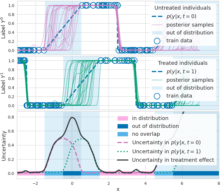
How can we identify covariate shifts and violations of overlap in individual-level causal inference? For this, we draw on Bayesian neural networks (BNNs): In probabilistic modelling, predictions may be assumed to come from a graphical model \(p(\mathrm{y} \mid \mathbf{x}, \mathrm{t},\mathbf{\omega})\) - a distribution over outputs (the likelihood) given a single set of parameters \(\mathbf{\omega}\). Considering a binary label \(\mathrm{y}\) given, for example, \(\mathrm{t} = 0\), a neural network can be described as a function defining the likelihood \(p(\mathrm{y} = 1 \mid \mathbf{x}, \mathrm{t} = 0, \mathbf{\omega}_0)\), with parameters \(\mathbf{\omega}_0\) defining the network weights. Different draws \(\mathbf{\omega}_0\) from a distribution over parameters \(p(\mathbf{\omega}_0 \mid \mathcal{D})\) would then correspond to different neural networks, i.e. functions from \((\mathbf{x}, \mathrm{t} = 0)\) to \(\mathrm{y}\). These are the purple curves in Fig. 1 (top). We discuss how to approximately but easily sample the posterior distribution \(p(\mathbf{\omega}_0 \mid \mathcal{D})\) in the paper.

Figure 1. How epistemic uncertainty detects lack of data. Top: binary outcome \(\mathrm{y}\) (blue circle) given no treatment, and different functions \(p(\mathrm{y} = 1|\mathbf{x}, \mathrm{t} = 0, \mathbf{\omega})\) (purple) predicting outcome probability (blue dashed line, ground truth). Functions disagree where data is scarce. Middle: binary outcome y given treatment, and functions \(p(\mathrm{y} = 1|\mathbf{x}, \mathrm{t} = 1, \mathbf{\omega})\) (green) predicting outcome probability. Bottom: measures of uncertainty/disagreement between outcome predictions (dashed purple and dotted green lines) are high when data is lacking. CATE uncertainty (solid black line) is higher where at least one model lacks data (non-overlap, light blue) or where both lack data (out-of-distribution / covariate shift, dark blue).
Figure 1 (top) illustrates the effects of a BNN’s parameter uncertainty in the range \(\mathbf{x} \in[−1, 1]\) (shaded region). While all sampled functions \(\mu^{\mathbf{\omega}_0} (\mathbf{x})\) with \(\mathbf{\omega}_0 \sim p(\mathbf{\omega}_0 \mid D, \mathrm{t} = 0)\) (shown in blue) agree with each other for inputs \(\mathbf{x}\) that are in-distribution (\(\mathbf{x} \in [−6, −1]\)) these functions make disagreeing predictions for inputs \(\mathbf{x} \in [−1, 1]\) because these lie out-of-distribution (OoD) with respect to the distribution that generates the training data, \(p(\mathbf{x} \mid \mathrm{t} = 0)\). This is an example of covariate shift for the function \(\mu^{\mathbf{\omega}_0}(\mathbf{x})\).
To avoid overconfident erroneous extrapolations on such OoD examples, we would like to indicate that the prediction \(\mu^{\mathbf{\omega}_0}(\mathbf{x})\) is uncertain. This uncertainty is called epistemic because it stems from a lack of data. We later show how to quantify it.
In Fig. 1, we illustrate that a lack of overlap constitutes a covariate shift problem.
- When \(p(\mathrm{t} = 1 \mid \mathbf{x}) \approx 0\), we face a covariate shift for \(\mu^{\mathbf{\omega}_1}(·)\) (because by Bayes rule \(p(\mathbf{x}^* \mid \mathrm{t} = 1) \approx 0\)), as shown in the middle panel.
- When \(p(\mathrm{t} = 1 \mid \mathbf{x}) \approx 1\), we face a covariate shift for \(\mu^{\mathbf{\omega}_0}(·)\) as shown in the top panel.
- And when \(p(\mathbf{x}) \approx 0\), we face a covariate shift for \(\widehat{\text{CATE}}^{\mathbf{\omega}_{0/1}} (\mathbf{x})\) (“out of distribution” in Fig. 1 (bottom)).
With this understanding, we can deploy tools for measuring epistemic uncertainty to address both covariate shift and non-overlap simultaneously.
Quantifying uncertainty about the treatment effect
Epistemic uncertainty measures disagreement between different plausible fits to the data. For a regression task such as estimating CATE, we quantify it as the variance:
\[\mathrm{Var}\left[\widehat{\text{CATE}}^{\mathbf{\omega}_{0/1}} (\mathbf{x})\right]=\mathop{\text{Var}}_{p(\mathbf{\omega}_0,\,\mathbf{\omega}_1 \mid \mathcal{D})} \left[\mu^{\mathbf{\omega}_1}(\mathbf{x})-\mu^{\mathbf{\omega}_0}(\mathbf{x})\right].\]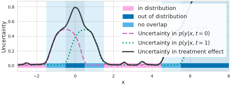
Figure 2. Measures of uncertainty/disagreement between outcome predictions (dashed purple and dotted green lines) are high when data is lacking. CATE uncertainty (solid black line) is higher where at least one model lacks data (non-overlap, light blue) or where both lack data (out-of-distribution / covariate shift, dark blue).
In Fig 2., when overlap is not satisfied for \(\mathbf{x}\), the uncertainty in the treatment effect \(\text{Var}[\widehat{\text{CATE}}^{\mathbf{\omega}_{0/1}} (\mathbf{x})]\) is large because at least one of \(\text{Var}_{\mathbf{\omega}_0}\left[\mu^{\mathbf{\omega}_0}(\mathbf{x})\right]\) and \(\text{Var}_{\mathbf{\omega}_1}\left[\mu^{\mathbf{\omega}_1}(\mathbf{x})\right]\) is large. Similarly, under a regular covariate shift \((p(\mathbf{x})\approx 0)\), both will be large.
We use this uncertainty and estimate it directly by sampling from an approximate posterior \(q(\mathbf{\omega}_0, \mathbf{\omega}_1 \mid \mathcal{D})\). There exists a large suite of methods we can leverage for this task, surveyed by Gal. Here, we use Monte Carlo Dropout because of its high scalability, ease of implementation, and state-of-the-art performance [4, 5, 6, 7]. However, our approach can be used with other approximate inference methods such as MCMC. Gal & Ghahramani have shown that we can simply add Dropout with L2 regularization in each of \(\mathbf{\omega}_0\), \(\mathbf{\omega}_1\) during training and then sample from the same dropout distribution at test time to get samples from \(q(\mathbf{\omega}_0,\, \omega_1 \mid \mathcal{D})\).
While most neural methods for causal inference can easily be equipped with epistemic uncertainty in this way, the Causal Effect Variational Autoencoder is more complicated. We show how to modify it in our paper.
Withholding automatic recommendations for points with high epistemic uncertainty - experimental evaluation
If there is insufficient knowledge about an individual, and a high cost for making errors, it may be preferable to withhold the treatment recommendation. In practice, we would withhold when the epistemic uncertainty exceeds a certain threshold, e.g. chosen to conform with public health guidelines. In our experiments, we instead sweep over different thresholds.
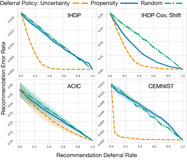
Figure 3: Plotting recommendation error rates against the proportion of recommendations deferred. We compare the epistemic uncertainty deferral policy (orange dashed lines) to propensity (blue solid lines) and random (green dash-dot line) deferral policies. We see that the uncertainty based policy leads to lower recommendation error rates for the IHDP, IHDP Covariate Shift, ACIC 2016, and CEMNIST datasets.
Baseline. When using the estimated propensity score \(p(\mathrm{t}=1 \mid \mathbf{x})\) for deferring recommendations, a simple policy is to specify a threshold \(\epsilon_0\) and defer points that do not satisfy eq. (4) with \(\epsilon = \epsilon_0\). More sophisticated standard guidelines were proposed by Caliendo & Kopeinig. We call their method propensity trimming. Since overlap must be assumed for most causal inference tasks, trimming methods are enormously popular [12, 13, 14, 15, 16]. But they are often cumbersome and sensitive to a large number of ad hoc choices that we can avoid by using epistemic uncertainty instead. Propensity trimming might be both too conservative, e.g. deferring points with low propensity where we actually have a good idea for how \(\mu_1\) would behave, and not conservative enough, e.g. not deferring cases where propensities are close to 0.5 but there is very high uncertainty regarding the outcome. Finally, the propensity score cannot in general identify points where covariate shift has occurred.
In our paper we show that propensity trimming can also be worse than random deferring as it does not consider that uncertainty is also modulated by the availability of data on points similar to \(\mathbf{x}\).
By using epistemic uncertainty, we can defer fewer points while achieving higher accuracy, as shown in Figure 3.
Table 1: Comparing epistemic uncertainty, propensity trimming, and random rejection policies for IHDP, IHDP Covariate Shift, and ACIC 2016 and with uncertainty-equipped SOTA models. 50% or 10% of examples set to be rejected and errors are reported on the remaining test-set recommendations. The epistemic uncertainty policy leads to the lowest errors in CATE estimates (in bold).
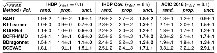
Epistemic uncertainty consistently outperforms propensity-based deferral across a range of uncertainty-aware neural models for causal inference (T-Learner, TARNet, CFRNet, Dragonnet, and CEVAE) and BART. It also gracefully handles situations with covariate shift as we demonstrate on IHDP.
Since causal inference is often needed in high-stakes domains such as medicine, we believe it is crucial to effectively communicate uncertainty and refrain from providing ill-conceived predictions. We hope that uncertainty-aware causal models will help realize personalized treatment recommendations by making them safer.
We hope to see you at our NeurIPS 2020 poster session and please check out the paper. If you are interested in running the above experiments, or evaluating your methods using the same datasets, please checkout our GitHub.
Acknowledgements
This paper would not have been possible without the support of many people. We would especially like to thank all anonymous reviewers, along with Lisa Schut, Milad Alizadeh, and Clare Lyle for their time, effort and valuable feedback. Thanks to Jose Medina for his help typesetting this blogpost.